Including systematic uncertainties to a model

[David_Vannerom]

Hello,

I am trying to add systematic uncertainties to a model. The model itself is trivial, the signal and background PDF’s are uniform at each value of the signal parameter, see the attached code.

compute_limits_example.py (7.5 KB)

The output from this code is the following plot:

You can see at lines 113-115, I have tried to replace the uniform distribution for the background by a Gaussian distribution to include the systematics. The result is the following:

The uncertainty bands get larger, but the limit itself gets better, which I don’t understand. My question is then: is the way I include the systematic uncertainties the correct way?

Thanks!

[jonas]

Hi @David_Vannerom,

sorry for the late reply, I understand that this is a follow up on Upper limits as a function of signal parameter

First of all the general idea: systematic uncertainties are implemented as additional nuisance parameters that are constrained by some auxiliary information. So in your case, the nuisance parameter is nbkg, and your constraint is a Gaussian distribution around some expected value with 10 % uncertainty, if I understand correctly.

Where you get it wrong is that you define this auxiliary Gaussian over the mass, and not nbkg. You should define an additional Gaussian for nbkg for your systematic constraint, and then multiply this on top of your existing model with RooProdPdf as explained in this tutorial.

In your script, this would look like

# Add nuisance parameter for background systematic constraint    
bkg_constr = ROOT.RooGaussian("bkg_constr", "bkg_constr", nbkg,
                 ROOT.RooFit.RooConst(bg), ROOT.RooFit.RooConst(0.1*bg)) 

# The  model for the counting experiment.    
model_noconstr = ROOT.RooAddPdf("model_noconstr", "model_noconstr",
                     ROOT.RooArgList(sig, bkg), ROOT.RooArgList(nsig, nbkg))
# The final model for the counting experiment with systematic constraints.
model = ROOT.RooProdPdf("model", "model",
                        ROOT.RooArgList(model_noconstr, bkg_constr))

That’s how you implement your background bg expectation with 10 % uncertainty.

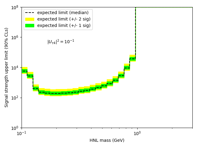
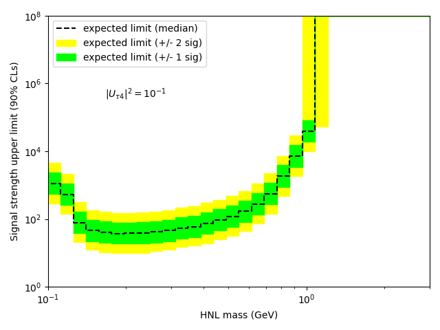
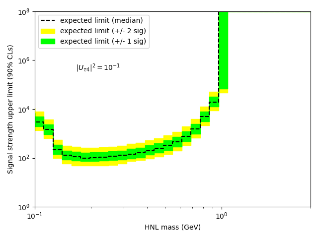
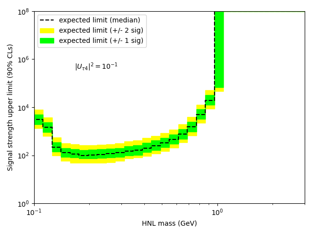
If you do that, you will indeed see that your limit improves (which was already the case in your original post, but only by chance I think). Why is that? In your fit that you based on my toy example from the previous thread, there was actually no background constraint included. I’m sorry that the example was so minimalist. Instead, the example just had a nbkg parameter that was completely floating and not constrained by any prediction. This is of course not a meaningful measurement, and the only power that this “analysis” had was to tell you that the signal can’t be more than the observed number of events, without subtracting the background. That’s also why your initial Brazilian plot in the other thread had this funny shape: if the nsig parameter was smaller than the expected observed number of events, your p-value was just flat 0.5, before dropping of.

So when you consider your Gaussian nkbg prediction with the 10 % uncertainty, you will improve your upper limit and have a meaningful analysis.

By the way, you can also check out how your analysis would perform if your background prediction is perfect and you have no systematic uncertainty: just fix your background parameter with nbkg.setConstant(True) and don’t pass any nuisance parameters to the model config with conf.SetNuisanceParameters(ROOT.RooArgSet()). That’s also a good sanity check. If your constraints are correctly implemented, your limits will be somewhere between the fixed-background case and the completely unconstrained case you started with.

I hope this makes sense to you, as always feel free to ask follow-up questions. I’ll try to answer them in time now!

Cheers,
Jonas

[David_Vannerom]

Hello Jonas,

Thanks a lot!

I have done the exercise to compare the three following scenarios: floating nbg, fixed nbg (to its expected value) and constrained nbg with a Gaussian (10% uncertainty):

I’m a little puzzled by the fact that the “no uncertainty” and “10% uncertainty” plots (the two last ones) are almost exactly the same. They are not, as you can see if you have a closer look at a few bins. Given that the expected number of background events is much larger than the expected number of signal events, I would expect an uncertainty on the BG to have a large impact, right? On the other hand, this corresponds to what I would expect for the signal, given the very low number of events.

[jonas]

Cool, that looks good! If your number of background events is small, the 10 % uncertainty will indeed not have a large impact because it’s dominated by the statistical uncertainty.

[David_Vannerom]

Hello Jonas,

I’ve got a question regarding the statistical uncertainty. In order to produce these plots, I have not used a number of events for the signal and the background, but rather a rate (number of events/unit time), which is much smaller. But whether I use a rate or a number of events, the ratio between the signal and background expectations stays the same (the multiplication factor is the same for both). My question concerns the treatment of the statistical uncertainty when using a rate: does the width of the uncertainty bands change if I multiply the signal and the bg by the same factor? Also, what if I add a systematic uncertainty: will it have the same impact regardless of an overall multiplication factor on the signal and background expectations (I insist on the fact that they always stay in a constant ratio)?

Thanks!