Hi, @Byungchul_Yu !
Regarding ROOT versions, it seems that the log-likelihood evaluation code is the same for versions from v6.30.02 to 6.40.02.
To get definitive results, I’ve decided to run a small numerical experiment.
Theoretical setup
Consider a histogram with two bins and a model predicting mean number of events in each bin \mu.
Fix true value \mu_0.
First bin gets number of events
y_1 \sim \mathrm{Poisson}(\mu_0).
Model prediction for the first bin is \mu.
Fix true value of a scale factor s_0.
The second bin gets weighted number of events
y_2 \sim \mathrm{Poisson}(\mu_0/s_0) \times s_0.
In case of 0 < s_0 < 1 the second bin will get larger amount of events \mu_0/s_0 with small weights s_0.
Note that model prediction for mean number of events for the second bin is \mu too.
Let’s denote objective function D to minimize for this problem as
D = k_1 \, \Delta\ell_1^{\mathrm{Poisson}} + k_2 \, \Delta\ell_2^{\mathrm{Poisson}}
where k_i are arbitrary weights.
Estimator for \mu is
\hat{\mu} = \mathrm{argmin}\,D(\mu)
Let’s derive it assuming that y_i are large enough to not hit parameter boundary \mu = 0:
\begin{align}
\frac{d}{d\mu}D(\mu) &=
\frac{d}{d\mu} \sum_i k_i \Delta\ell_i^{\mathrm{Poisson}} =
\\ &=
\frac{d}{d\mu} \sum_i k_i \left( -y_i \log\frac{\mu}{y_i} + \mu - y_i \right) =
\\ &=
\sum_i k_i \left( -\frac{y_i}{\mu} + 1 \right) = 0
\end{align}
From there it follows that
\hat{\mu} = \frac{\sum_i k_i y_i}{\sum_i k_i}
which is greater than zero under assumption that y_i > 0.
Natural choices for k_i as a function of s_i = \frac{\sigma_i^2}{y_i} from this topic are limited to
k_i =
\begin{cases}
s_i, & \text{apparent from ROOT source code} \\
1, & \text{Poisson likelihood} \\
\frac{1}{s_i}, & \text{Scaled Poisson likelihood}
\end{cases}
Theoretical Estimator Performance
Note that by definition of how y_i are generated s_i are constant
s_1 = \frac{\sigma_1^2}{y_1} = \frac{\sum_{j=1}^{j=y_1} 1}{\sum_{j=1}^{j=y_1} 1} = 1,
s_2 = \frac{\sigma_2^2}{y_2} = \frac{\sum_{j=1}^{j=y_2} s_0^2}{\sum_{j=1}^{j=y_2} s_0} = s_0,
and hence k_i = \text{const}
Taking expectation and variance of estimator, we get
\mathrm{E}\hat{\mu} = \frac{k_1 \mathrm{E}y_1 + k_2 \mathrm{E}y_2}{k_1 + k_2} =
\frac{k_1 \mu_0 + k_2 \mu_0/s_0 \times s_0}{k_1 + k_2} = \mu_0
\mathrm{Var}\,\hat{\mu} = \frac{k_1^2 \mathrm{Var}\,y_1 + k_2^2 \mathrm{Var}\,y_2}{(k_1 + k_2)^2} =
\frac{k_1^2 \mu_0 + k_2^2 \mu_0/s_0 \times s_0^2}{(k_1 + k_2)^2} = \mu_0 \frac{k_1^2 + k_2^2 s_0}{(k_1 + k_2)^2}
We see that all estimators are unbiased, and choice of k_i affects only variance.
\mathrm{Var}\,\hat{\mu} = \mu_0 \times
\begin{cases}
\frac{1 + s_0^3}{(1 + s_0)^2}, & \text{ROOT source code} \\
\frac{1 + s_0}{4}, & \text{Poisson deviance} \\
\frac{s_0}{1 + s_0}, & \text{Scaled Poisson deviance}
\end{cases}
It can be shown that for s_0 > -1
\frac{s_0}{1 + s_0} < \frac{1 + s_0}{4} < \frac{1 + s_0^3}{(1 + s_0)^2}
From another perspective, just by summing all events without weights we expect to see
N \approx \mu_0 (1 + 1/s_0)
events in total, and on the other hand
N = y_1 + y_2/s_0,
and we get rule of thumb estimator
\tilde{\mu} = \frac{y_1 + y_2/s_0}{1 + 1/s_0},
which coincides with Scaled Poisson estimator.
Numerical check
Let’s introduce two performance metrics under repeated toy experiments:
\text{bias} = \text{Mean}(\hat{\mu}) - \mu_0
\text{overdispersion} = \text{RMS}(\hat{\mu}) \left/ \sqrt{\frac{\mu_0 s_0}{1 + s_0}} \right.
the latter motivated by the fact that Scaled Poisson estimator should show the least variance.
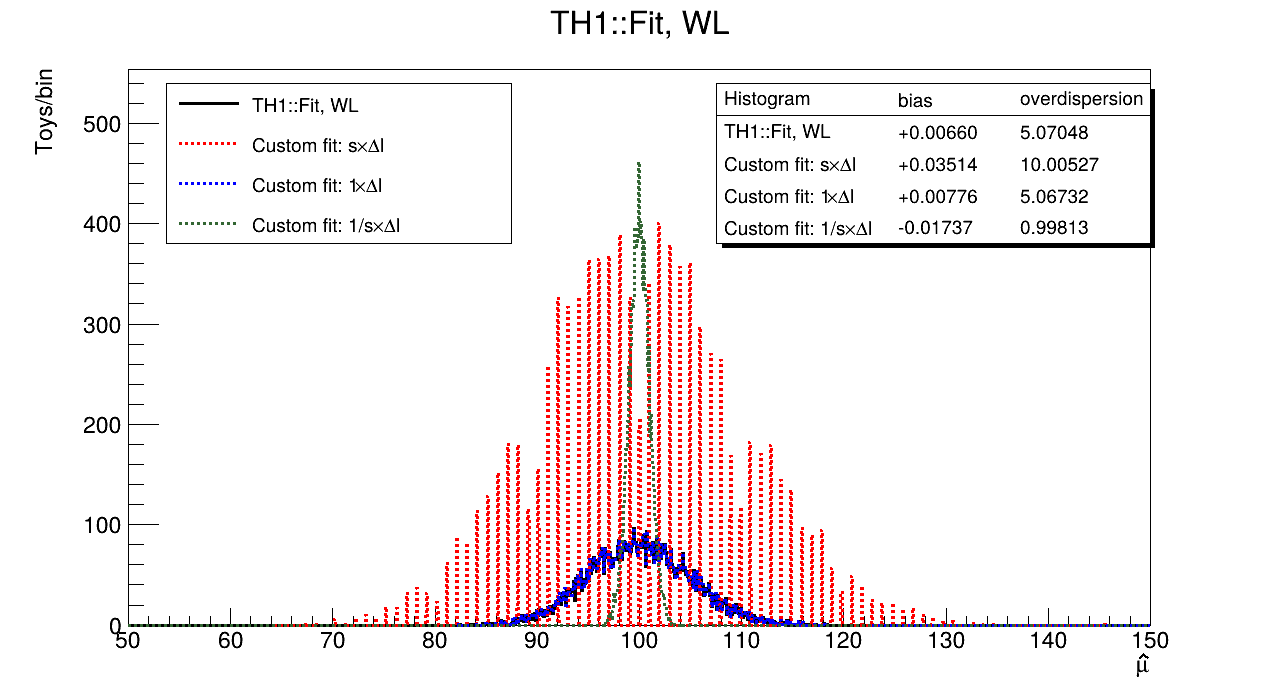
I’ve written a script to compare distributions of \hat{\mu} given by TH1::Fit with WL option, and given by the three choices of the objective function.
True values are \mu_0 = 100, s_0 = 1/100 and 10000 toys are generated.
fit_WL.cxx (9.8 KB)
Results
Discussion
It can be clearly seen that ROOT performs similarly to objective function
or option 2, k_i = 1, despite the fact that as I see from the source code that ROOT’s objective function to minimize is
s_i^2 \,
\Delta\ell_i^{\mathrm{SPD}}
=
s_i \Delta\ell_i^{\mathrm{Poisson}}
which is very confusing for me. It is likely that I interpreted the source code incorrectly.
Nevertheless, it is also clear that option 3, k_i = 1/s_i objective function
\Delta\ell_i^{\mathrm{SPD}}
=
\frac{1}{s_i} \Delta\ell_i^{\mathrm{Poisson}}
outperforms ROOT TH1::Fit with WL option in this specific setting.
This can be explained by the fact that s_0 \ll 1, and neglecting this factor exaggerates variance of the ROOT estimator.
Despite the fact that scale factor affects likelihood term for the second bin by two orders of magnitude, variance of the estimator is degraded only approximately by factor of 5, which is fully explained by overdispersion formula:
\sqrt{\frac{1 + s_0}{4} \times \frac{1 + s_0}{s_0}} = \frac{1 + s_0}{2\sqrt{s_0}} = 5.05
For s_0 = 1/T and large T, overdispersion degrades asymptotically quadratically, \propto \sqrt{T}
The effect of non-constant, random event weights on estimator performance is unknown at this point, but it is intuitively appealing that variance in weights inside bin would introduce additional overdispersion.
In practice I’d expect that effective statistics is large, meaning that s_0 \lesssim 1, and overdispersion does not degrade significantly.
For non-linear models I claim that mis-specification of weights for likelihood terms might emphasize wrong local minima or assign more weight to a steeper gradient descent direction, introducing bias and amplifying variance of resulting estimator.
The latter can be corrected by sandwich covariance estimator though.
Conclusion
The numerical check on this toy problem converged to @Byungchul_Yu suspicion that ROOT minimizes Poisson deviance.
In the simple setting with two bins and constant event weights there exists an estimator which minimizes Scaled Poisson deviance and outperforms ROOT’s TH1::Fit with WL option.
Dear @Byungchul_Yu , please check if the results of the scripts are similar for you.
I would like also to humbly invite other experts, @jonas and @StephanH to the discussion.