Weighted log likelihood estimation for low statistics binned histogram

Hello,

I have weighed binned histogram and at later time, the bin contents contains low statistics.
I have two pieces of information (bin contents which are weighted by some values ranging from 0.1 to 0.8 and bin errors which are obtained by the error propagation). The bin contents (counts) follows a model and this model includes 5-parameters. I want to extract those parameters exactly as much as I can.

I have performed the weighted log likelihood estimation to estimate those parameters by using “WL” option. I think the results look good, but I really want to cross check if those results are reasonable through the goodness of fit. In the meantime, what I really want to know is how “WL” option works to estimate the parameters by using those two pieces information in more detail.

Would you mind giving me some advice on that? Also, i want to know the exact form of probability mass function of the weighted poisson distribution in my case.

Thank you

Hi Byungchul,

I add in the loop the expert, @moneta , and suggest that in the meantime you check the code (this is a great advantage of ROOT, an open source tool) to see if it does exactly what you expect.

Cheers,
Danilo

Hello,

The WL option can be used to fit weighted histogram, representing sum of weighted counts, i.e. in case you gave a Poisson process giving {w_i} counts in each bin.
You can find a theoretical explanations in this paper, https://arxiv.org/pdf/1309.1287.pdf
ROOT implements what is described in paragraph 3: the approximation with a scaled Poisson distribution.
In your case, it seems to me you have an histogram where the bin content follows a particular model. If the error is computed from error propagation, you are basically using a Normal approximation. I think in this case it would be more appropriate doing a standard least-square fit, the default in ROOT and not use option “WL”.

Best regards

Lorenzo

Thank you for looping the expert to me. Sure, I have checked my code several times!

Hi Lorenzo, thanks for your feedback and providing me with the theoretical paper.

I think it would be better to explain my situation a bit more detail to get your advice more correctly.
First, I have 650 thousand weighted histograms and I am planning to extract one of the parameters from those histograms and perform the time-resolved analysis. This is my whole analysis plan.

Each histogram contains about 35000 counts, but due to some systematics, the total events in my fit range are approximately 25000 counts. The total number of bins is about 4000 in this fit range. However these events follows exponential decay with respect to particle’s lifetime. Thus, after 2000th bins, there are a few counts in the bin contents. So, basically, if I consider the earlier bins, you’re right. those follow the normal distribution, but I am planning to set the specific fit ranges to get more statistical power and it includes lots of bins including low statistics (the number of counts in each bin are less than 10 after 1500th bins).

Each bin in the histograms are weighted by particular different numbers which are obtained by the error propagation because all the events (counts) are considered identical, independent data.

I have already performed the standard least-square fit and, but I got the biased fit results due to the low statistics. However, when I performed the weighted log likelihood estimation by using the option “WL”, I got more correct central value for the fit parameters and the results were not biased. This is why I started to change the fit method from the chi2 fit to the likelihood method.

As far as I know and I talked with other co-workers, our original counts follows poisson distribution with the different expected counts, but we weighted each bin contents with different values ranging from 0.1 to 0.9. The weights are function of particle’s energy but it is not known.

I really want to confirm how “WL” option is operating and how they calculate the fit uncertainty, and what is the exact form of log likelihood estimation formula, etc.

Would you mind giving me some advice on that?

Hi,

I would need to understand your problem better to see if the WL option is correct for your case.
As described in the paper linked above, this is a weighted likelihood fit, where the PDF used for each bin is not the standard Poisson, but an approximated one, where the number of effective entries (a real number, not an integer) is used. The number of effective entries is given by the (sum of weight)^2/(sum of weight^2) and the scale factor for each bin is (sum of weight^2)/(sum of weight). You can also check this in the code implementing this here:

Best,

Lorenzo

Hi @moneta,

I’ve also been digging into the WL fit, and I was wondering how ROOT actually calculates the weighted negative log-likelihood (NLL) to be minimized.
According to the code you shared, the NLL is computed through lines 1567-1586 with the WL option.

The only difference between the standard L fit is that you multiply weight = (error * error) / y; (Line 1577) to the NLL for each bin (leaving aside when the bin content (y) is 0 for the moment).
So I ran a quick test to compare the NLL for the L fit and NL fit.
Here are my codes:

    int nbins = 10;
    double c_true = 4.5;

    TH1F* h = new TH1F("h", "", nbins, 0, nbins);
    TF1* f = new TF1("f", "[0]", 0, nbins);

    TRandom3* rng = new TRandom3(seed);

    for (int i=0; i<nbins; i++) {
        for (int j=0; j<rng->Poisson(c_true); j++) {
            h->Fill(i, rng->Rndm());
        }
    }
    
    TFitResultPtr r1 = h->Fit("f", "QSR0");     // Chi-square fit
    TFitResultPtr r2 = h->Fit("f", "QSRL0");    // Likelihood fit
    TFitResultPtr r3 = h->Fit("f", "QSRWL0");   // Weighted likelihood fit

    TGraph* g1 = new TGraph();
    TGraph* g2 = new TGraph();
    TGraph* g3 = new TGraph();
    double theta_start = 0.1;
    double theta_end = 3;
    
    f->FixParameter(0, 0);
    for (double theta=theta_start; theta<theta_end; theta+=0.01)
    {
        f->SetParameter(0, theta);
        
        double nll = 0;
        for (int i=0; i<nbins; i++) {
            double y_i = h->GetBinContent(i+1);
            double e_i = h->GetBinError(i+1);
            double sum_of_weights = y_i;
            double sum_of_weight_squared = e_i * e_i;
            double scale_factor = sum_of_weight_squared / sum_of_weights;
            
            nll += scale_factor * (y_i * (log(y_i) - log(theta)) + theta - y_i); // Weighted likelihood fit.
        }

        TFitResultPtr r1_ = h->Fit("f", "QSRL0");
        g1->SetPoint(g1->GetN(), theta, r1_->MinFcnValue());
        TFitResultPtr r2_ = h->Fit("f", "QSRWL0");
        g2->SetPoint(g2->GetN(), theta, r2_->MinFcnValue());
        g3->SetPoint(g3->GetN(), theta, nll);
    }

    std::cout << "\nChi-squared fit" << std::endl;
    std::cout << "Fit\t" << r1->Parameter(0) << "\t" << r1->ParError(0) << std::endl;

    std::cout << "\nLikelihood fit" << std::endl;
    std::cout << "Fit\t" << r2->Parameter(0) << "\t" << r2->ParError(0) << std::endl;

    std::cout << "\nWeighted likelihood fit" << std::endl;
    std::cout << "Fit\t" << r3->Parameter(0) << "\t" << r3->ParError(0) << std::endl;

    TCanvas* c = new TCanvas("c", "", 800, 600);
    g1->SetLineColor(kBlue);
    g1->SetLineWidth(2);
    g1->Draw("apl");
    g2->SetLineColor(kRed);
    g2->Draw("same");
    g3->SetLineColor(kGreen);
    g3->Draw("same");

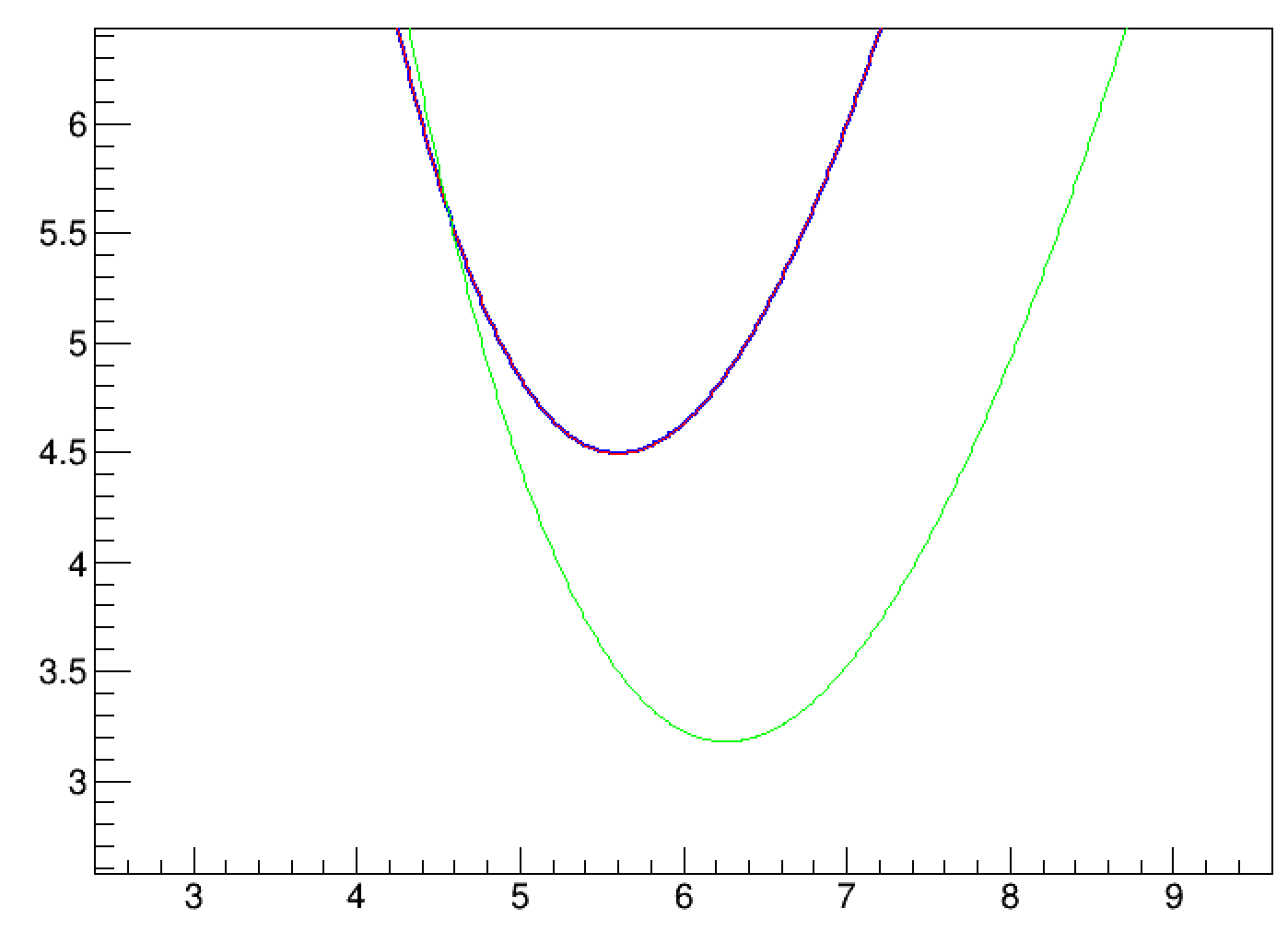
I made a simple histogram with weighted Poisson variables and fitted it with a constant (theta).
g1 is the NLL vs. theta in the likelihood fit (blue),
g2 is the NLL vs. theta in the weighted likelihood fit (red), and
g3 is the NLL vs. theta from the same formula used in ROOT for the WL fit (green).

I expected that red and green are the same, and they are different from blue.
However, the resulting plot shows that red is the same as blue.

It suggests that your NLL for the WL fit is exactly the same as that for the L fit, in contrast to what’s implemented in lines 1567-1586 of your code, which confused me.

And it is unclear to me how the WL fit calculates the covariance matrix.

This could be a separate question, but I also have a doubt about the NLL for the weighted Poisson case.
I followed the references you put and derived that the scale factor should be divided, not multiplied, in the likelihood.
So I believe the line 1577 should be weight = y / (error * error); instead of weight = (error * error) / y;

To sum up, I have 3 questions:

  1. The NLL in the WL fit seems to be exactly the same as that in the L fit, as opposed to what’s written in the source code. There might be a bug.
  2. Still, the variance of parameters from the WL fit is different from the L fit. How the covariance matrix is computed in the WL case?
  3. The weight weight = (error * error) / y; seems to be corrected to weight = y / (error * error);

Best regards,
On

Hi Lorenzo,

I spent some time to think about WLLE with the stuff that you provided me.
What I really want to know for WLLE is exactly the same as what bigstraon9 wrote down above.
I think it will be of great help to me if the answers to the questions bigstraon9 asked become clear.
I am looking forward to answering the questions he asked above, I am waiting.

Thank you so much.

With warm regards,
Byungchul Yu

Hello @bigstaron9

Thank you for looking into this. You are correct, the difference between a L fit in ROOT and a WL fit is only in the computation of the covariance matrix, the central result value (minimum of the likelihood is the same. You can see this in the code at line 1588 of the link above.
In the WL you use a scale Poisson weighted by a weight W, but you need to use as observed events in the poisson not Y (the bin count or sum of the weight in each bin) but the number of effective entries: (y^2/error^2). And you need to scale also the number of expected events in each bin. The end result is exactly the same likelihood.

For computing the covariance matrix, the procedure described in F. James book, Statistical Method in Experimental Physics, par. 8.5.2 is used. With this procedure the covariance matrix is corrected from the computation of teh covariance matrix where the likelihood is computed using the weight square. This is sone in the code block starting at line 1566.

The weight (or scale factor and not to be confused from the single event weight used to fill the histogram) to use for each bin in the likelihood is computed using the relation:

Bin content y = weight * number of effective entries

Given that the number of effective entries is (y*y)/(error*error) , the weight is then
(error * error)/y

I hope I have answered all 3 questions, if not , please let me know

Lorenzo

Hi @moneta

Thank you for your explanation and correction.
I think I totally understood the likelihood of being maximized in the case of the WL fit.

            double y_i = h->GetBinContent(i+1);
            double e_i = h->GetBinError(i+1);
            double sum_of_weights = y_i;
            double sum_of_weight_squared = e_i * e_i;
            double scale_factor = sum_of_weight_squared / sum_of_weights;
            double num_effective = y_i * y_i / sum_of_weight_squared;
            double scaled_theta = theta * y_i / sum_of_weight_squared;
            
            nll += scale_factor * (num_effective * (log(num_effective) - log(scaled_theta)) + scaled_theta - num_effective); // Weighted likelihood fit.

which reduces to the exact same likelihood for the case of the likelihood fit.

Still, I haven’t quite gotten the idea of how to compute the covariance matrix.
I looked up and read Sec. 8.5.2 of the reference carefully, and my logic went as follows.

  1. W' in Eq. (8.43) is the log-likelihood, so we have these correspondences: 1/e_i in Eq. (8.43) is the scale factor defined in the above code, ln(P_i) in Eq. (8.43) is num_effective * (log(num_effective) - log(scaled_theta)) + scaled_theta - num_effective in the above code (this is ‘negative’ log-likelihood, though, so probably corresponds to -ln(P_i).)
  2. The remaining computations are straightforward, at least for this case, where my model is just a constant fit (theta). I computed D_1' and D_2' on page 197 of Sec. 8.5.2 and successively the variance of my fit parameter theta using the last equation on page 196.
  3. The resulting variance reads \sigma_\theta^2 = \sum_i {scale_factor_i * y_i} / N^2.
    I didn’t find anything wrong with my calculation, but the result was not consistent with what was found in the WL fit.

Your code starting at line 1566 computes the likelihood using the weight squared. And you are saying that this likelihood is NOT used to compute the central value, but only for the covariance matrix, did I understand right? I guess you are numerically computing D_2 (or H’_{kl} in Eq. (8.47)) with this likelihood.
Please let me know if there’s anything I am still misunderstanding.
Thanks for your help.

Best,
On

Hi,

yes, what is done is to compute numerically H and H’ the two Hessian matrices (inverse of covariance) numerically as done in eq. 8.47 and then apply eq. 8.48 for the resulting covariance.
However, this is not fully correct, as reported in this recent paper, https://arxiv.org/pdf/1911.01303.pdf
This is now implemented in RooFit using the AsymptoticError option for general unbinned fit.

Best,

Lorenzo

Hi @moneta,

Thanks a lot for clarifying.
My analytic calculations agree perfectly with what the fitter found.
In Eq. (8.47), there are typos: 1/N shouldn’t be there inside square brackets.
Everything makes sense now.

I also looked up the paper you referred to: https://arxiv.org/pdf/1911.01303.pdf
If it’s more accurate, can it also be applicable to the binned weighted likelihood fits?
Although I’m not familiar with sWeights, so I’ll have to see whether it’s applicable to our analysis first.

Best,
On

Hello,

I will have to study if the new asymptotic procedure is applicable for binned fits. I would presume it, especially in the case of a large number of bins.

Lorenzo

This topic was automatically closed 14 days after the last reply. New replies are no longer allowed.