Hi all,
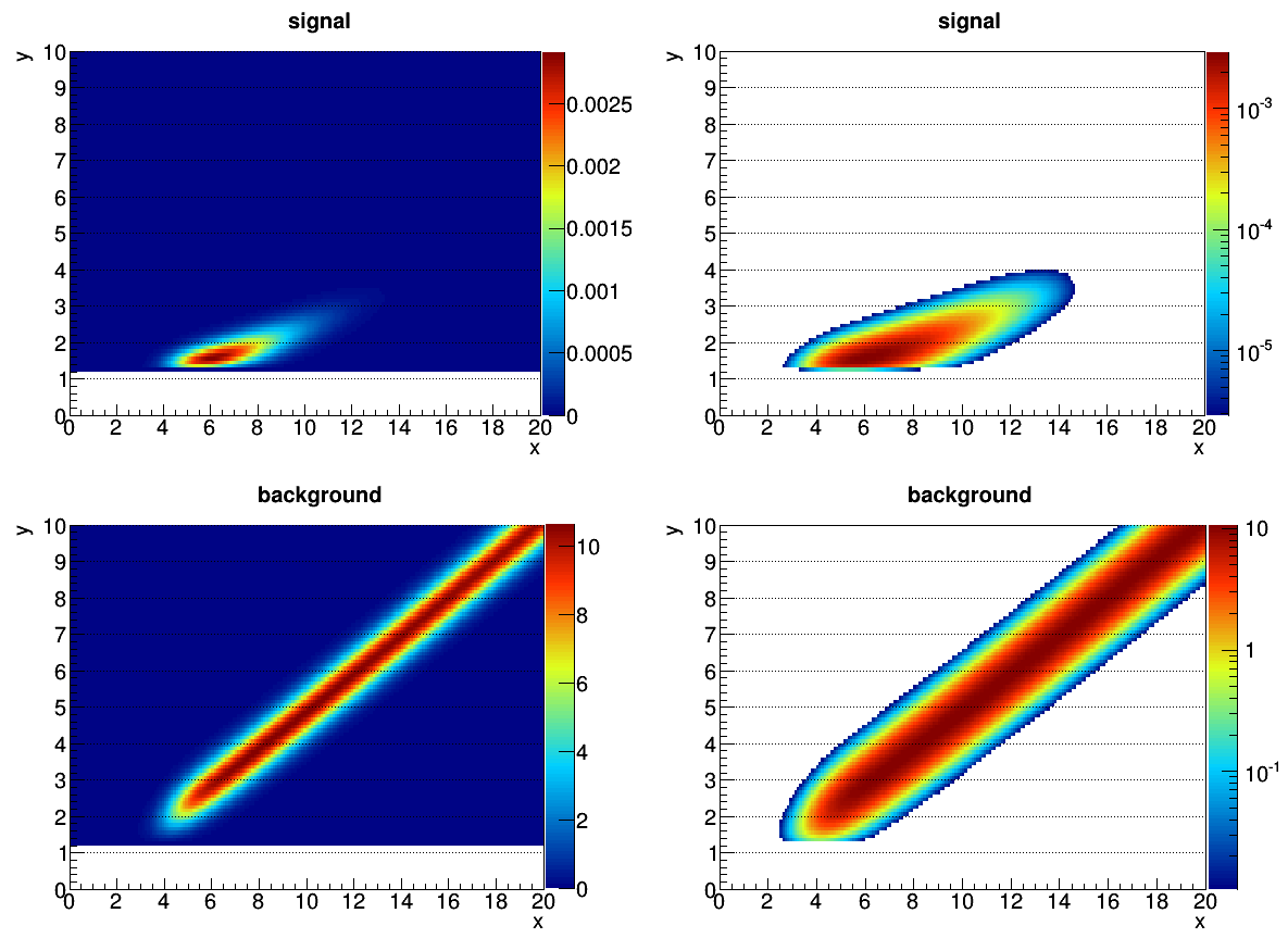
I have problems with a 2 dimensional extended maximum likelihood fit including a signal and a background. A large fraction of the fits return a number of signal events which is completely unphysical. Both signal and background are constant PDFs without any additional shape parameters. They are created from histograms as RooHistPdfs (see plot 1 with normal and log scale for each histogram) and have only a small overlap, i,e, they are well separated.
The only fit parameters therefore are the number of signal and background events, N_sig and N_bkgd.
For the moment I’m testing the model to determine the discrimination power. To do that I set the signal PDF to zero events and the background PDF to i.e. 100 events. From this I create 10,000 monte carlo toy sets and fit the total PDF. The idea was that (the width of) the N_signal distribution tells me about the discrimination power of my PDF model.
Now to the problem:
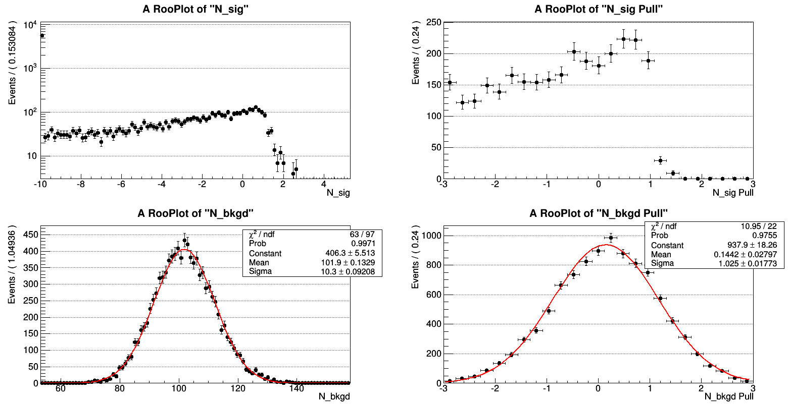
As plot 2 shows, an overwhelming fraction of fits doesn’t converge around N_sig = 0 (as one should expect because no signal component should be present in the toy event samples) but extends all the way down to the lower limit of the N_sig parameter (no matter if that is set to -10 or -500!). So apparently small fluctuations into the signal PDF are fitted as expected but under fluctuations lead to completely unphysical results for the number of signal events.
Limiting the signal to positive values gives a best fit of N_sig = 0.0 for most of the fits, which is not a distribution itself.
Attached is a root file with the two histograms used to create the PDFs as well as the python script with a minimal working example of the problem.
I would be very grateful for any comments and suggestions to help me understand and maybe solve this problem. Thanks,
lukash
Plot 1:
Plot 2:
Minimal working example:
#!/usr/bin/env python
"""Minimal working example

"""

from ROOT import *
from ROOT import RooFit
from ROOT.RooFit import *


x = RooRealVar('x', 'x', 0., 20)
y = RooRealVar('y', 'y', 0., 10)


HistFile = TFile('histograms.root', 'READ')


# Get background histogram and create PDF
BkgdHist = HistFile.Get('background')
BkgdDataHist = RooDataHist('bkgd_datahist', 'bkgd_datahist', RooArgList(x, y), BkgdHist)
BkgdPdf = RooHistPdf('bkgd_pdf', 'bkgd_pdf', RooArgSet(x, y), BkgdDataHist)
N_bkgd = RooRealVar('N_bkgd', 'N_bkgd', 100., 0., 200.)


# Get signal histogram and create PDF
SigHist = HistFile.Get('signal')
SigDataHist = RooDataHist('sig_datahist', 'sig_datahist', RooArgList(x, y), SigHist)
SigPdf = RooHistPdf('sig_pdf', 'sig_pdf', RooArgSet(x, y), SigDataHist)
N_sig = RooRealVar('N_sig', 'N_sig', 0., -10., 20.)


# Total PDF consisting of signal and background
TotalPdf = RooAddPdf('total_pdf', 'total_pdf', RooArgList(BkgdPdf, SigPdf), RooArgList(N_bkgd, N_sig) )


# Monte Carlo study
MCStudy = RooMCStudy(TotalPdf, RooArgSet(x, y), Extended(kTRUE), FitOptions(Save(kTRUE), Verbose(kFALSE)) )
MCStudy.generateAndFit(10000)


# Plot parameter and pull distribution of the Monte Carlo Study
canvas = TCanvas()
canvas.Divide(2, 2)

canvas.cd(1)
frame1 = MCStudy.plotParam(N_sig)
frame1.Draw()

canvas.cd(2)
frame2 = MCStudy.plotPull(N_sig)
frame2.Draw()

canvas.cd(3)
frame3 = MCStudy.plotParam(N_bkgd)
frame3.Draw()

canvas.cd(4)
frame4 = MCStudy.plotPull(N_bkgd)
frame4.Draw()
minimal_working_example.py (1.45 KB)
histograms.root (551 KB)