Total ionization and free electron fraction (FEF)

[pigerard]

Dear experts,

I’m trying to validate what Garfield output by comparing to some experimental values by 2 ways.

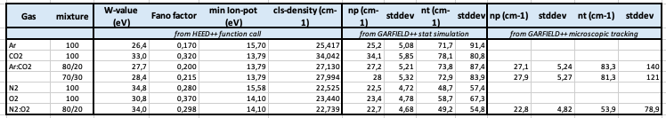
1. First one, I’m trying to get the correct number of total electrons from a ionizing particle (proton) at MIP (\beta\gamma = 3.3) using TrackHeed in N2/O2 (80/20) mixture (with a gas file I have generated) and in Ar/CO2 (80/20) (with the gas file in the examples) both at NTP. Comparing to tables found online and in lectures, the values I get are quite far.

Gas 1	n_p (cm^{-1})	n_t (cm^{-1})
O2	22	73
N2	10	56
Ar	23	94
CO2	35.5	91
—	—	—
N2/O2 (80/20)	12.4	59.4
Ar/CO2 (80/20)	25.5	93.4

On 1000 tracks of proton in a plane parallel geometry with a gap of 0.1cm I get for total electrons in:

• N2/O2 (80/20): 7.09 so 70.9 cm^{-1}
• Ar/CO2 (80/20): 6.10 so 61.0 cm^{-1}
• O2: 6.99 so 69.9 cm^{-1}

Is it normal to have such a big difference from the literature ? (I mean O2 is ok but the 2 mixtures are not so accurate).

Here is my full code

  const double gap = .1; // [cm]
  const double detectorXWidth = 10; // [cm] 
  const double detectorZWidth = 10; // [cm]
  const double vPlate = 500.; // [V]
  string particle = "proton";
  const double KineticEnergy = 230e6; // [eV] (230Mev or 230.e6 eV for proton therapy [eV])
  const double BetaGamma = 3.3;
  const unsigned int nTracks = 1000;
  //vector<string> gasFile = {"ar_80_co2_20_0T.gas", "IonMobility_Ar+_Ar.txt"};
  //vector<string> gasFile = {"air_merged.gas", "IonMobility_N2+_N2.txt", "IonMobility_O2-_air.txt"};
  vector<string> gasFile = {"pureOxygen_merged.gas", "IonMobility_O2-_O2.txt"};"IonMobility_O2-_air.txt"};
  //vector<string> gasFile = {"Hochhauser_N2_O2_100kPa.gas", "IonMobility_N2+_N2.txt", "IonMobility_O2-_air.txt"};
  
  // Gas
  MediumMagboltz gas;
  gas.LoadGasFile(gasFile[0]);
  const string path = getenv("GARFIELD_INSTALL");
  gas.LoadIonMobility(path + "/share/Garfield/Data/" + gasFile[1]);
  gas.LoadNegativeIonMobility(path + "/share/Garfield/Data/" + gasFile[2]);

  // Geometry
  ComponentAnalyticField cmp;
  cmp.SetMedium(&gas);
  cmp.AddPlaneY( 0., 0.);
  cmp.AddPlaneY(gap, vPlate, "s");

  // Sensor
  Sensor sensor;
  sensor.SetArea(-detectorXWidth/2, 0, -detectorZWidth/2, detectorXWidth/2, gap, detectorZWidth/2);
  sensor.AddComponent(&cmp);
  sensor.AddElectrode(&cmp, "s");
  const double tstep = 1;
  const double tmin = -0.5 * tstep;
  const unsigned int nbins = 1000;
  sensor.SetTimeWindow(tmin, tstep, nbins);


  // Track
  TrackHeed track;
  track.SetSensor(&sensor);
  track.SetParticle(particle);
  //track.SetKineticEnergy(KineticEnergy);
  track.SetBetaGamma(BetaGamma);
  //track.Initialise(&gas, true);
  
  // Avalanche for the electrons
  AvalancheMicroscopic aval; 
  aval.SetSensor(&sensor);

  // Drift for the ions
  AvalancheMC drift;
  drift.SetSensor(&sensor);
  

  vector<int> vec_cluster;
  vector<int> vec_totalElectron;
  vector<int> vec_multiplicationElectron;
  vector<int> vec_leftedElectron;
  vector<int> vec_attachedElectron;
  vector<int> vec_collectedElectron;


  int flag_electronStatus = 0; // flag for the electron status in case of wierd status

  for (unsigned int j = 0; j < nTracks; ++j) {
    cout << "Track " << j+1 << "/" << nTracks << endl;
    //sensor.NewSignal();
    track.NewTrack(0, 0, 0, 0, 0, 1, 0); // x0, y0, z0, t0, dx0, dy0, dz0

    int ncluster = 0; // number of clusters
    int totalElectron = 0; // primary + delta electrons
    int multiplicationElectron = 0; // primary + delta electrons after multiplication
    int leftedElectron = 0; // electrons who left the drift area
    int attachedElectron = 0; // electrons attached to a molecule/atom
    int collectedElectron = 0;  // electrons collected by the electrode

    for (const auto& cluster : track.GetClusters()) {
      ncluster ++;
      totalElectron += cluster.electrons.size();
      for (const auto& electron : cluster.electrons) {
        
        aval.AvalancheElectron(electron.x, electron.y, electron.z, electron.t, 0.1, 0, 0, 0); // x0, y0, z0, t0, e0, dx0, dy0, dz0
        const unsigned int np = aval.GetNumberOfElectronEndpoints();
        double xe1, ye1, ze1, te1, e1;
        double xe2, ye2, ze2, te2, e2;
        int status;
        multiplicationElectron += np;
        for (unsigned int j = 0; j < np; ++j) {
          aval.GetElectronEndpoint(j, xe1, ye1, ze1, te1, e1, xe2, ye2, ze2, te2, e2, status);
          //drift.DriftIon(xe1, ye1, ze1, te1);
          if (status == -7) {
            attachedElectron ++;
            //drift.DriftNegativeIon(xe2, ye2, ze2, te2);
          }
          if (status == -5) collectedElectron ++;
          if (status == -1) leftedElectron ++;
          if (status == -3 || status == -8 || status == -16 || status == -17) flag_electronStatus +=1;
        }
      }
    }
  vec_cluster.push_back(ncluster);
  vec_totalElectron.push_back(totalElectron);
  vec_multiplicationElectron.push_back(multiplicationElectron);
  vec_leftedElectron.push_back(leftedElectron);
  vec_attachedElectron.push_back(attachedElectron);
  vec_collectedElectron.push_back(collectedElectron);
  }

  double mean_cluster = accumulate(vec_cluster.begin(), vec_cluster.end(), 0.0) / nTracks;
  double mean_totalElectron = accumulate(vec_totalElectron.begin(), vec_totalElectron.end(), 0.0) / nTracks;
  int absolute_multiplicationElectron = accumulate(vec_multiplicationElectron.begin(), vec_multiplicationElectron.end(), 0.0) - accumulate(vec_totalElectron.begin(), vec_totalElectron.end(), 0.0);
  double mean_multiplicationElectron = accumulate(vec_multiplicationElectron.begin(), vec_multiplicationElectron.end(), 0.0) / nTracks;
  double mean_leftedElectron = accumulate(vec_leftedElectron.begin(), vec_leftedElectron.end(), 0.0) / nTracks;
  double mean_attachedElectron = accumulate(vec_attachedElectron.begin(), vec_attachedElectron.end(), 0.0) / nTracks;
  double mean_collectedElectron = accumulate(vec_collectedElectron.begin(), vec_collectedElectron.end(), 0.0) / nTracks;

  auto stop = chrono::high_resolution_clock::now();
  auto duration = chrono::duration_cast<chrono::seconds>(stop - start);
  time_t now = time(0);
  char* dt = ctime(&now);
  
  
  cout << endl;
  cout << "     " << dt << endl;
  cout << "Gap size:              " << gap << " cm" << endl;
  cout << "Voltage:               " << vPlate << " V" << endl;
  cout << "Particle:              " << particle << endl;
  cout << "Kinetic energy:        " << KineticEnergy << " eV/c" << endl;
  cout << "Gas file:              " << gasFile[0] << endl;
  cout << "                       " << gasFile[1] << endl;
  cout << "                       " << gasFile[2] << endl;
  cout << endl;
  cout << "     " << "Mean on " << nTracks << " different tracks" << endl;
  cout << "Clusters:                                      " << mean_cluster << endl;
  cout << "Total electrons:                               " << mean_totalElectron << endl;
  cout << "Total electrons after avalanche:               " << mean_multiplicationElectron << endl;
  cout << "Multiplication (absolute):                     " << "+" << absolute_multiplicationElectron << endl;
  cout << "Ratio of attached electrons:                   " << double (mean_attachedElectron/mean_multiplicationElectron) << endl;
  cout << "Ratio of collected electrons:                  " << double (mean_collectedElectron/mean_multiplicationElectron) << endl;
  cout << "Ratio of electrons who left the drift area:    " << double (mean_leftedElectron/mean_multiplicationElectron) << endl;
  if (flag_electronStatus > 0) cout << "/!\\ There was a problem computing the electron status /!\\"<< endl;
  cout << endl;
  cout << "Time taken by computation: " << duration.count() << " seconds" << endl << endl;

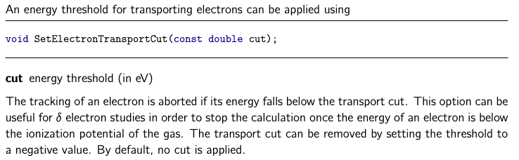
I also tried to turn off the simulation of the \delta electrons (secondary electrons) with track.DisableDeltaElectronTransport() add simulate those secondary electrons with AvalancheMicroscopic and the primaries electorns in input.

    for (const auto& cluster : track.GetClusters()) {
      ncluster ++;
      primaryElectron += cluster.electrons.size();
      for (const auto& electron : cluster.electrons) {
        aval.AvalancheElectron(electron.x, electron.y, electron.z, electron.t, electron.e, electron.dx, electron.dy, electron.dz); // x0, y0, z0, t0, e0, dx0, dy0, dz0
        const unsigned int np = aval.GetNumberOfElectronEndpoints();
        double xe1, ye1, ze1, te1, e1;
        double xe2, ye2, ze2, te2, e2;
        int status;
        totalElectron += np;
        for (unsigned int j = 0; j < np; ++j) {
          aval.GetElectronEndpoint(j, xe1, ye1, ze1, te1, e1, xe2, ye2, ze2, te2, e2, status);
          //drift.DriftIon(xe1, ye1, ze1, te1);
          if (status == -7) {
            attachedElectron ++;
            //drift.DriftNegativeIon(xe2, ye2, ze2, te2);
          }
          if (status == -5) collectedElectron ++;
          if (status == -1) leftedElectron ++;
          if (status == -3 || status == -8 || status == -16 || status == -17) flag_electronStatus +=1;
        }
      }
    }

With this method the computation takes longer and I have significant different results. Which method is more correct ?

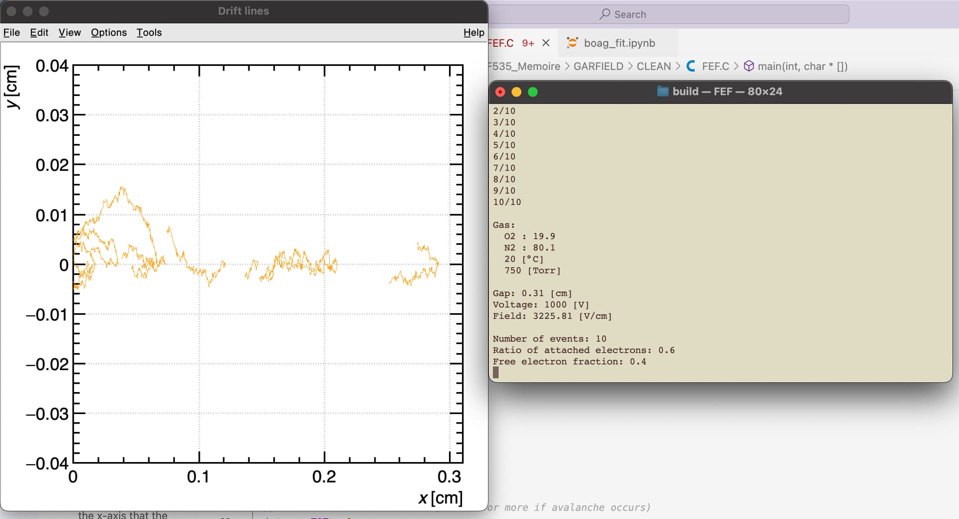
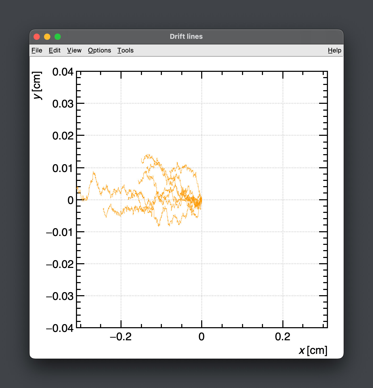
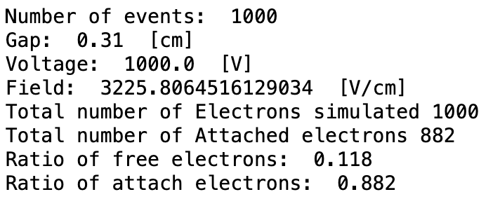
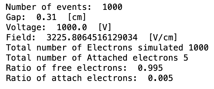
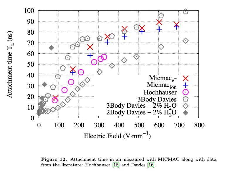
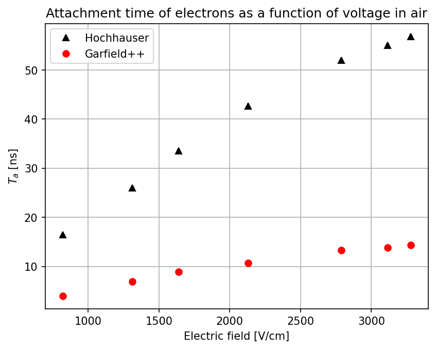
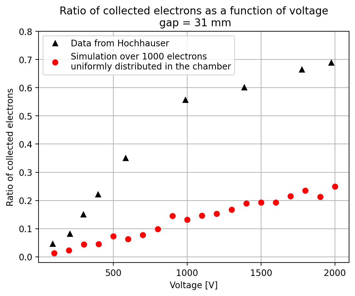
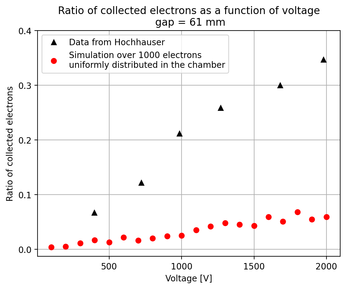
2. The second way is by comparing the number of collected electrons with the free electron fraction (i.e. the fraction of electron who escape the recombination and reach the electrode as free electron) measured by Hochhauser that show J.W. Boag in is paper of 1996 ( DOI 10.1088/0031-9155/41/5/005). In his paper we have 2 plots for gaps of 0.31 cm and 0.61 cm both in dry syntethic air and laboratory air.

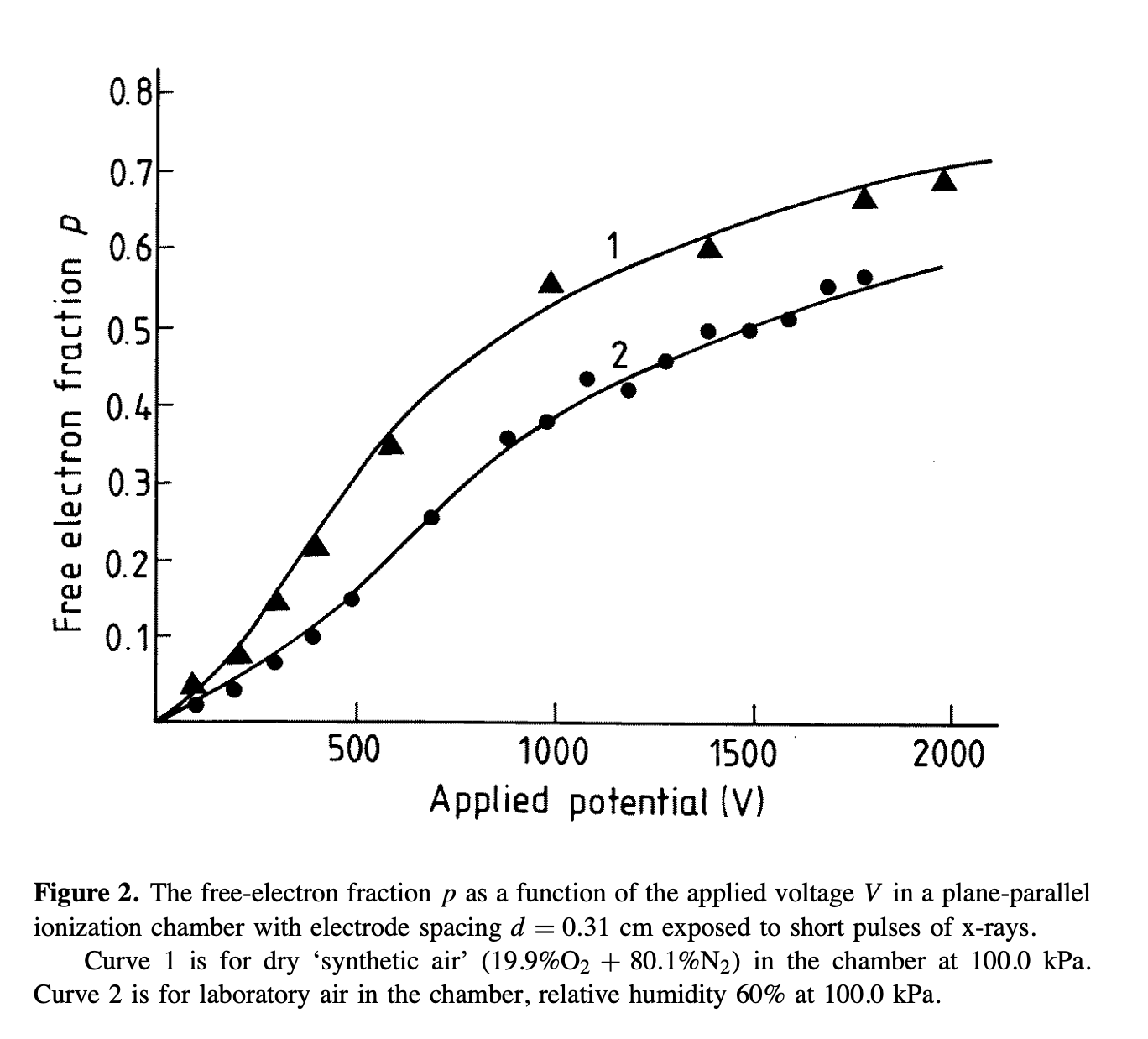
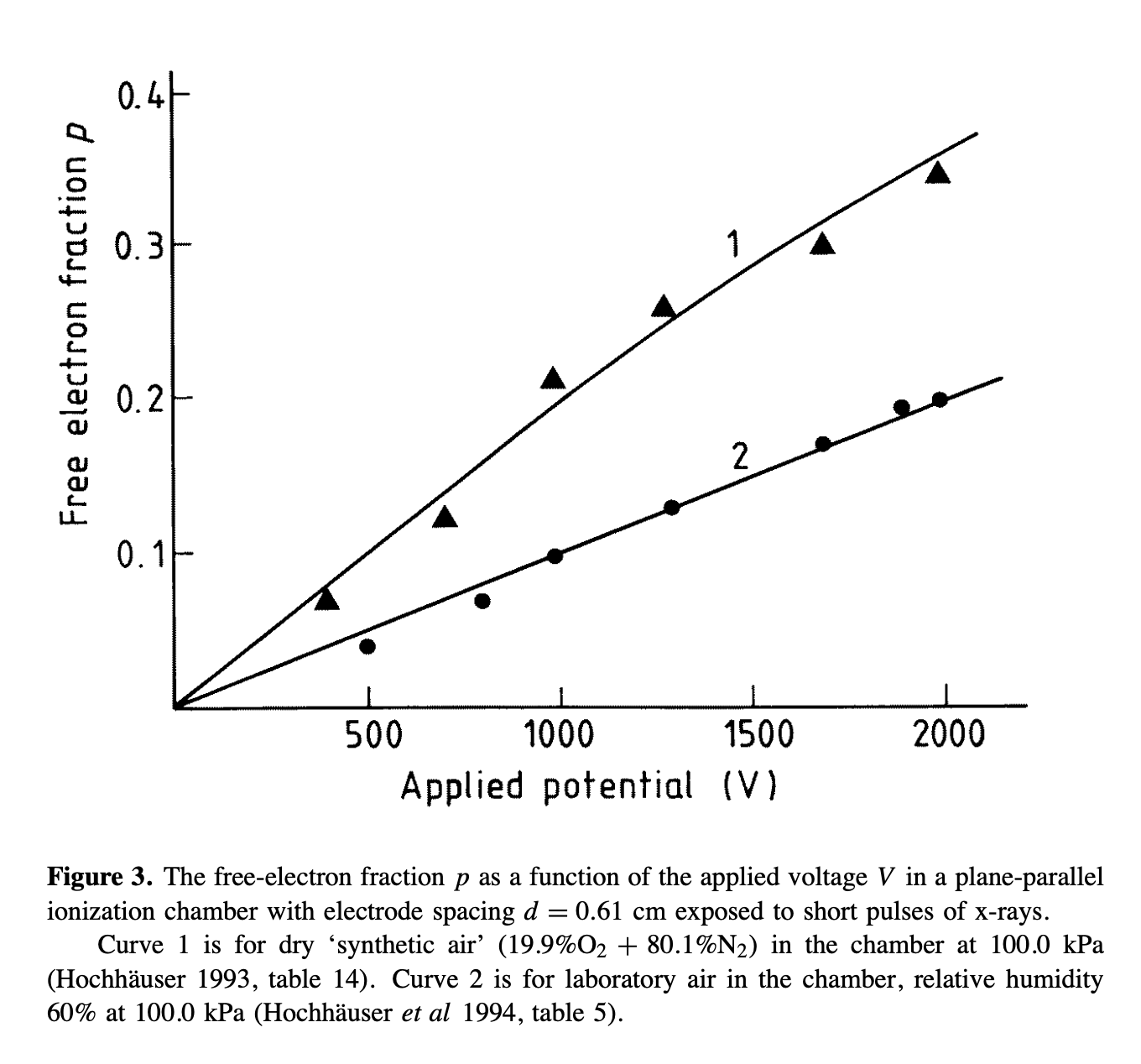
I have generate a new gas file matching the synthetic air at 100 kPa to compare. With this code, and for both gaps i tried get the value of the collected electrons by putting electrons uniformly distributed in the plane parallel geometry at different potential but as you seen the results from Garfield are not matching Hochhauser measurement.

Thanks a lot for your help.

Pierre

vector<double> vPlateValues = {100,  200,  300,  400,  500,  600,  700,  800,  900, 1000, 1100,
       1200, 1300, 1400, 1500, 1600, 1700, 1800, 1900, 2000};

  for (double vPlate : vPlateValues) {

    const double gap = .31; // [cm]
    const double detectorXWidth = 5; // [cm] 
    const double detectorZWidth = 5; // [cm]
    const unsigned int nElectrons = 1000;
    vector<string> gasFile = {"Hochhauser_N2_O2_100kPa_NO_HUMID.gas",
                              "IonMobility_N2+_N2.txt",
                              "IonMobility_O2-_air.txt"};

    // Gas
    MediumMagboltz gas;
    gas.LoadGasFile(gasFile[0]);
    const string path = getenv("GARFIELD_INSTALL");
    gas.LoadIonMobility(path + "/share/Garfield/Data/" + gasFile[1]);
    gas.LoadNegativeIonMobility(path + "/share/Garfield/Data/" + gasFile[2]);

    // Geometry
    ComponentAnalyticField cmp;
    cmp.SetMedium(&gas);
    cmp.AddPlaneY( 0., 0.);
    cmp.AddPlaneY(gap, vPlate, "s");

    // Sensor
    Sensor sensor;
    sensor.SetArea(-detectorXWidth/2, 0, -detectorZWidth/2, detectorXWidth/2, gap, detectorZWidth/2);
    sensor.AddComponent(&cmp);
    sensor.AddElectrode(&cmp, "s");
    const double tstep = 1;
    const double tmin = -0.5 * tstep;
    const unsigned int nbins = 1000;
    sensor.SetTimeWindow(tmin, tstep, nbins);

    // Avalanche for the electrons
    AvalancheMicroscopic aval;
    aval.SetSensor(&sensor);

    // Drift for the ions
    AvalancheMC drift;
    drift.SetSensor(&sensor);



    vector<int> vec_totalElectron;
    vector<int> vec_leftedElectron;
    vector<int> vec_attachedElectron;
    vector<int> vec_collectedElectron;
    int flag_electronStatus = 0; // flag for the electron status in case of weird status

    for (unsigned int j = 0; j < nElectrons; ++j) {
      cout << "Electron " << j+1 << "/" << nElectrons << endl;

      int totalElectron = 0; // primary + delta electrons + avalanche if any
      int leftedElectron = 0; // electrons who left the drift area
      int attachedElectron = 0; // electrons attached to a ion
      int collectedElectron = 0;  // electrons collected by the electrode

      double x0 = -detectorXWidth/2 + detectorXWidth * RndmUniform();
      double y0 = gap * RndmUniform();
      double z0 = -detectorZWidth/2 + detectorZWidth * RndmUniform();

      aval.AvalancheElectron(x0, y0, z0, 0, 0.1, 0, 0, 0); // x0, y0, z0, t0, e0, dx0, dy0, dz0
      const unsigned int np = aval.GetNumberOfElectronEndpoints();
      double xe1, ye1, ze1, te1, e1;
      double xe2, ye2, ze2, te2, e2;
      int status;
      totalElectron += np;
      for (unsigned int j = 0; j < np; ++j) {
        aval.GetElectronEndpoint(j, xe1, ye1, ze1, te1, e1, xe2, ye2, ze2, te2, e2, status);
        //drift.DriftIon(xe1, ye1, ze1, te1);
        if (status == -7) {
          attachedElectron ++;
          //drift.DriftNegativeIon(xe2, ye2, ze2, te2);
        }
        if (status == -5) collectedElectron ++;
        if (status == -1) leftedElectron ++;
        if (status == -3 || status == -8 || status == -16 || status == -17) flag_electronStatus +=1;
      }
      
    vec_totalElectron.push_back(totalElectron);
    vec_leftedElectron.push_back(leftedElectron);
    vec_attachedElectron.push_back(attachedElectron);
    vec_collectedElectron.push_back(collectedElectron);
    }

    double mean_totalElectron = accumulate(vec_totalElectron.begin(), vec_totalElectron.end(), 0.0) / nElectrons;
    double mean_leftedElectron = accumulate(vec_leftedElectron.begin(), vec_leftedElectron.end(), 0.0) / nElectrons;
    double mean_attachedElectron = accumulate(vec_attachedElectron.begin(), vec_attachedElectron.end(), 0.0) / nElectrons;
    double mean_collectedElectron = accumulate(vec_collectedElectron.begin(), vec_collectedElectron.end(), 0.0) / nElectrons;

    // Time
    auto stop = chrono::high_resolution_clock::now();
    auto duration = chrono::duration_cast<chrono::seconds>(stop - start);
    time_t now = time(0);
    char* dt = ctime(&now);
    
    cout << endl;
    cout << "     " << dt << endl;
    cout << "Gap size:              " << gap << " cm" << endl;
    cout << "Voltage:               " << vPlate << " V" << endl;
    cout << "Gas file:              " << gasFile[0] << endl;
    cout << "                       " << gasFile[1] << endl;
    cout << "                       " << gasFile[2] << endl;
    cout << endl;
    cout << "     " << "Mean on " << nElectrons << " different tracks" << endl;
    cout << "Total electrons:                               " << mean_totalElectron << endl;
    cout << "Ratio of attached electrons:                   " << double (mean_attachedElectron/mean_totalElectron) << endl;
    cout << "Ratio of collected electrons:                  " << double (mean_collectedElectron/mean_totalElectron) << endl;
    cout << "Ratio of electrons who left the drift area:    " << double (mean_leftedElectron/mean_totalElectron) << endl;
    if (flag_electronStatus > 0) cout << "/!\\ There was a problem computing the electron status /!\\"<< endl;
    cout << endl;
    cout << "Time taken by computation: " << duration.count() << " seconds" << endl << endl;

[vpadulan]

Dear @pigerard ,

Thanks for reaching out to the forum! Maybe @hschindl could help you with your question.

Cheers,
Vincenzo

[Piet]

Dear @pigerard

Excellent question, validation is a cornerstone of scientific work. Now, I think you have to be a bit careful in selecting the tables found online, in lectures, in books and in papers, as they can vary wildly vary. I would stick with some trusted reference works such as Particle Detection with Drift Chambers [1] or the Particle Physics Reference Library [2], you can access both through the CERN library.

Now your question on validation of the simulation of primary ionization regards exactly work done by @hschindl in his PhD thesis [3], so I would recommend you have a look at chapter 4. Also Igor Smirnovs HEED++ paper [4] discusses the validation and both find “fair” agreement, of the order of ~10% between simulation and experimental data. I find some values in your table a bit dubious (e.g. np for N2). I was also not 100% convinced of your heed simulations, so I ran a few myself, based on the Edep.C example of garfield++ [5] and here are my results (I attach some distributions below):

As you can see there are some differences between some textbooks and HEED, but they are rather contained, see also the discussion in @hschindl thesis. I also run with Microscopic Tracking (MT) and I disabled the Delta Electron Transport algorithm in HEED, and I observe that MT gives me about 10% higher values for the total number of electrons (n_T). I was able to maintain the computing time very reasonable implementing an energy cutoff on the electron transport, as suggested in the garfield++ manual [6]:

I would consider this 10% difference between the HEED delta electron transport algorithm and the microscopic tracking as an estimate of the uncertainty to assign to n_T.

For what concerns your 2nd question, I would believe that you do not correctly “tag” your electrons. I do not know exactly the difference between status -1 (particle left drift area) and -5 (particle not inside a drift medium), I would have to look into the source code to understand. I would think that for remaking the plots of the free electron fraction you compare the total number of electrons liberated by a charged particle to that same number with the attached electrons subtracted, because that is the only process that matters here. Alternatively I would believe counting status -1 and -5 together (and assuming you do not have calculation errors (status -3) or electrons lost due to time window or energy cut (status -16,-17) you would find the same numbers.

NB. for the simulation of Heed (TrackHeed class) or Microscopic Tracking (AvalancheMicroscopic class) you do not need to provide a gasfile. A gas file is required for AvalancheMC or DriftLineRKF simulation as it requires the knowledge of the Townsend, Attachment and Diffusion coefficients that vary as function of the Electric and Magnetic Field.

[1] Particle Detection with Drift Chambers | SpringerLink
[2] Particle Physics Reference Library: Volume 2: Detectors for Particles and Radiation | SpringerLink
[3] Microscopic Simulation of Particle Detectors - CERN Document Server
[4] Redirecting
[5] Heed | Garfield++
[6] https://garfieldpp.web.cern.ch/garfieldpp/documentation/UserGuide.pdf

Primary-Ionization-240424.pdf (213.0 KB)
Primary-Ionization-MicroTrk-240424.pdf (58.3 KB)

[hschindl]

Hi,
just a few additions to Piet’s already very comprehensive explanations:

• For the purposes of validating the primary ionisation observables I would indeed skip the avalanche simulation and use TrackHeed only, like in the “edep” example in the repository (C++ version, Python version).
• The average cluster density (n_p) is a quite well defined quantity, while for “n_T” things are a bit more fuzzy: as can be seen from the set of plots that Piet attached, the distribution of ionisation electrons has a long tail, so there is a significant difference between the mean and the most probable value. The mean is also affected to some extent by the geometry (for instance, high-energy delta electrons might escape a chamber). Also both mean and MPV depend of course on the particle momentum.
• I just had a look at the PDG review and the experimental values for n_p you have in your table are quite similar to what’s quoted there. Might be worth clarifying with the authors what definition they use, what measurements the numbers are based on, etc. For genuine “MIPs” the numbers given in the PDG seem high to me.

I have to read the second question more carefully, but one thing that might be worth mentioning is that Garfield++ does not consider electron-ion recombination.

[pigerard]

Hi @hschindl and @Piet ,
First of all thanks a lot for your answers. They are very helpfull for me. My first question is much more clear and checking the 2 references [1] and [2] from @Piet gave me more confidence of the outputs of Garfield.

However I’m working on the FEF in the air and even with your suggestions I couldn’t get the results from Hochhausser. Computing the ratio as the attached electrons over all the electrons of the avalanche (even if the avalanche doesnt occure) does not change my previous results.

Here is a piece of my new code

  // Make a medium
  MediumMagboltz gas("o2", 19.9, "N2", 80.1);
  gas.SetTemperature(273.15 + 20);
  gas.SetPressure(760.);

  // Thickness of the gas gap [cm] and voltage [V]
  constexpr double gap = .31;
  constexpr double voltage = 1000.;

  // Make a component
  ComponentConstant cmp;
  cmp.SetArea(0., -10., -10., gap, 10., 10.);
  cmp.SetMedium(&gas);
  double field = voltage / double(gap);
  cmp.SetElectricField(field, 0., 0.);

  // Make a sensor
  Sensor sensor;
  sensor.AddComponent(&cmp);

  // Avalanche class
  AvalancheMicroscopic aval;
  aval.SetSensor(&sensor);


  // Total number of electrons (nEvents or more if avalanche occurs)
  int nsumTOT = 0;
  // Total number of attached electrons
  int asumTOT = 0;
  const int nEvents = 1000;
  for (int i = 0; i < nEvents; ++i) {
    std::cout << i+1 << "/" << nEvents << " event" << "\n";
    // Initial position and direction 
    double x0 = gap * RndmUniform(), y0 = 0., z0 = 0., t0 = 0.;
    double dx0 = 1., dy0 = 0., dz0 = 0.;
    double e0 = .1;
    // number of electrons (1 or more if avalanche occurs)
    int nsum = 0;
    // number of attached electrons
    int asum = 0;
    aval.AvalancheElectron(x0, y0, z0, t0, e0, dx0, dy0, dz0);
    double xe1, ye1, ze1, te1, e1;
    double xe2, ye2, ze2, te2, e2;
    int status;
    // Loop over the electron avalanches.
    nsum = aval.GetNumberOfElectronEndpoints();
    for (int j = 0; j < nsum; ++j){
      aval.GetElectronEndpoint(j, xe1, ye1, ze1, te1, e1, xe2, ye2, ze2, te2, e2, status);
      if (status == -7) asum ++;
    }
    nsumTOT += nsum;
    asumTOT += asum;
  }
  double attachRatio = 1 - (asumTOT / (double)nsumTOT);

  std::cout << "Number of events: " << nEvents << "\n";
  std::cout << "Gap: " << gap << " [cm]" << "\n";
  std::cout << "Voltage: " << voltage << " [V]" << "\n";
  std::cout << "Field: " << field << " [V/cm]" << "\n";
  std::cout << "Ratio of attached electrons: " << attachRatio << "\n";

@hschindl you’have mentioned that Garfield++ doesn’t consider electron-ion. Do you think this could be the reason of such a big difference in my previous plots ?
In [A] p.84 and [B] p.65 it is shown that the electron-ion in air is negligible but also that it decreases as a function of the electric field. But in my comparison plots we see worst results at higher voltage.

Thank you a lot agin for your help.

Pierre

[A] Dosimetry of highly pulsed radiation fields|INIS
[B] Chambres d’ionisation en Protonthérapie et Hadronthérapie - TEL - Thèses en ligne

[Piet]

@pigerard maybe you can make an event display (viewdrift) for a single event to understand where all your electrons end up?

[pigerard]

Here is a view for 10 electrons

[hschindl]

Hi,
not sure if this is really the explanation, but one reason could be electrons that are backscattered to the cathode. As a test, can you make the gap twice as large and start the electron in the middle of the gap.

I think it should be enough to change the lines of code where you set up the “component” to this:

ComponentConstant cmp;
cmp.SetArea(-gap, -10., -10., gap, 10., 10.);
cmp.SetMedium(&gas);
double field = 2 * voltage / gap;
cmp.SetElectricField(field, 0., 0.);

As an aside (which has nothing to do with the issue you described): if you want to be more concise, you can also write the loop over the electron “endpoints” like this:

aval.AvalancheElectron(x0, y0, z0, t0, e0, dx0, dy0, dz0);
for (const auto& electron : aval.GetElectrons()) {
  ++nsum;
  if (electron.status == -7) ++asum;
}

[pigerard]

Hello @hschindl, I’m not sure to understand this test. Even if a double the potential when I double the gap in order to maintain the electric field the same (and so drift velocity), the time of drift of the electron will be greater because of the greater gap and then the attachement also will be greater and not comparable to the measurements.

Here is the result for a single gap and electrons put in the middle of the gap.

Gap: 0.31 [cm]
Voltage: 1000 [V]
Field: 6451.61 [V/cm]

Number of events: 1000
Ratio of attached electrons: 0.873
Free electron fraction: 0.127

Here te same for a double gap and electrons put also in he middle

Gap: 0.62 [cm]
Voltage: 2000 [V]
Field: 6451.61 [V/cm]

Number of events: 1000
Ratio of attached electrons: 0.992
Free electron fraction: 0.008

Here a ViewDrift of the double gap for 10 electrons

Thank you for your note about the loop over the electrons !

[hschindl]

Ah, sorry, I hadn’t read your previous post carefully enough. I thought you were using a fixed starting point of the electron.

I’ll try to run your example to make sure I can reproduce the results…

[Piet]

hi @pigerard @hschindl

I had a look at your code and implemented it in a SWAN jupyterworkbook that I shared with you.
I believe I am able to reproduce the results, for 1000V, I did not perform an entire scan. I ran it also for Ar:CO2 70:30 as I know that gasmixture better, and indeed there the result is more or less what I exprected: very low fraction of attachment.

Result for N2:O2 80.1:19.9 ::

Result for Ar:CO2 70:30 ::

So I would think the code is ok, but we should maybe look into the cross-sections and see whether the attachment cross section is reasonable. We would have to ask to some experts. Running the gas.PlotElectronCrossSections() command I get the following cross section plots (first one for N2, second one for O2):

What concerns the units, they do not quite agree with the garfieldpp website x-section plotter, I would expect the elastic cross sections to be around ~100Mbarn, what do you think @hschindl?

[pigerard]

Hello @Piet and @hschindl

I just tried another way to match the measurement from Hochausser. In his paper from 1994 [1] he measured the electron attachement time for multiple fields strength. Those results where validates by Boissonnat [2] here

Those measurement where took at 1000 hPa, 20 °C and in laboratory air with 60% rel. humidity. I approximate the air composition with (“o2”, 21.1, “Ar”, .9, “H2O”, 1., “N2”, 77.). I used only MediumMagboltz in order to get the value of the attachment coef. and drift velocity at those specific fields. Then, using the formula in Boissonnat’s paper [2]

T_a = \frac{1}{\eta~v_{e^-}}

I compared the results with Hochhauser’s one and again they clearly not fit.

[1] Hochhauser, E., Balk, O., Schneider, H., & Arnold, W. (1994). The significance of the lifetime and collection time of free electrons for the recombination correction in the ionometric dosimetry of pulsed radiation. Journal Of Physics. D, Applied Physics, 27(3), 431‑440. The significance of the lifetime and collection time of free electrons for the recombination correction in the ionometric dosimetry of pulsed radiation - IOPscience

[2] Boissonnat, G., Fontbonne, J., Colin, J., Remadi, A., & Salvador, S. (2016). Measurement of ion and electron drift velocity and electronic attachment in air for ionization chambers. arXiv (Cornell University). [1609.03740] Measurement of ion and electron drift velocity and electronic attachment in air for ionization chambers