Dear Pierre
My plot is showing the average energy of the electrons when they collide with a gas molecule in an electric field of 3.2kV/cm (1000V uniform over 0.31cm). You can make this plot easily when you run Microscopic Tracking by including the following lines after the initialization of an instance of the AvalancheMicroscopic class and before launching an electron:
hEnergy = ROOT.TH1F(“hEnergy”, “Electron energy”, 100, 0., 10.)
aval.EnableElectronEnergyHistogramming(hEnergy)
Indeed, another nice way to investigate this is by how you did it by looking at the endpoint energy of the electrons that end up attached. It would be better to have a histogram with logaritmic binning for that, starting at 0.1 eV and up to let’s say 10eV.
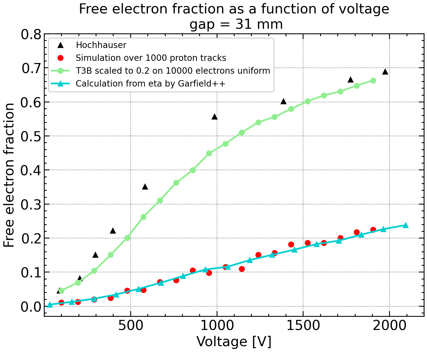
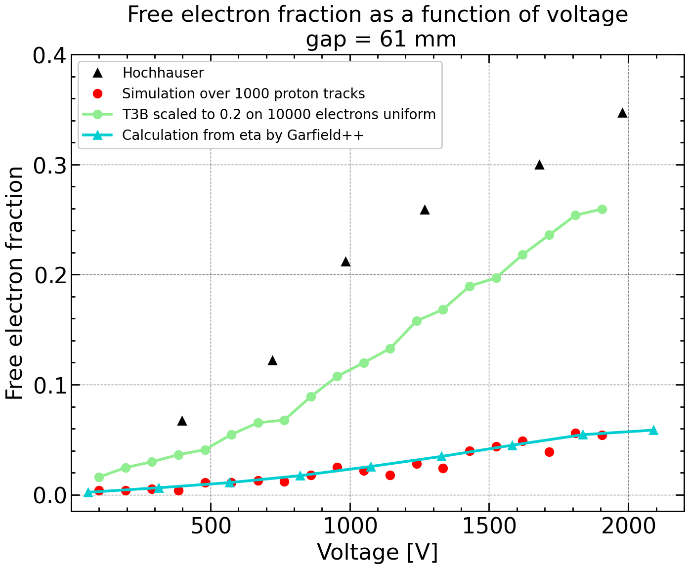
So I also set T3B to 0.199 in Magboltz/magboltz.f file for Oxygen gas and I ran a couple of simulations: one using microscopic tracking, another one using monte-carlo (avalancheMC) and I obtained much better agreement with your Hochhauser measurements (I attach my code below):
Microscopic Tracking:
MediumMagboltz::SetComposition: N2/O2 (80.1/19.9)
Electric Field: 3225.8064516129034 V/cm
Number of events: 1000
Microscopic Tracking: True
Gap: 0.31 [cm]
Voltage: 1000.0 [V]
Field: 3225.8064516129034 [V/cm]
Total number of Electrons simulated 1000
Total number of Attached electrons 490
Ratio of free electrons: 0.51
Ratio of attach electrons: 0.49
Monte-Carlo technique using macroscopic transport parameters:
MediumMagboltz::LoadGasFile:
Reading file n2_80p1_o2_19p9_magboltz_modified.gas.
Version 12.
Gas composition set to O2/N2 (19.9/80.1).
Electric Field: 3225.8064516129034 V/cm
Number of events: 1000
Microscopic Tracking: False
Gap: 0.31 [cm]
Voltage: 1000.0 [V]
Field: 3225.8064516129034 [V/cm]
Total number of Electrons simulated 1000
Total number of Attached electrons 564
Ratio of free electrons: 0.436
Ratio of attach electrons: 0.564
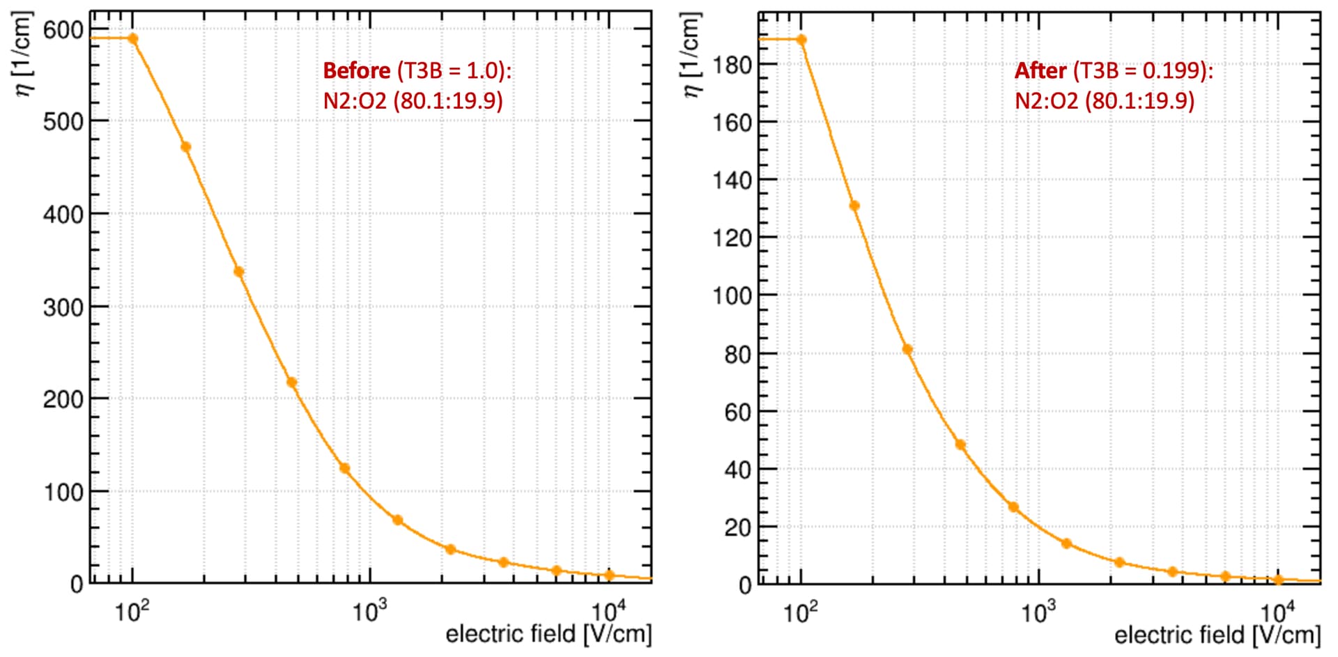
For running the Monte-Carlo technique I made first a gasfile that contains the macroscopic transport parameters. This is what I typically do if I would like to know these parameters to plot e.g. drift velocity, townsend coefficient, attachment coefficient. With the new gasfile (generated with T3B = 0.199) I find a much lower attachment coefficient:
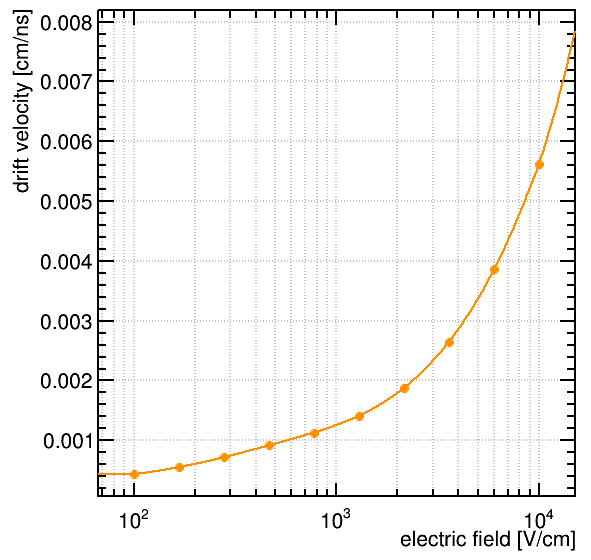
While I find for the drift velocity exactly the same curve (it is unaffected):
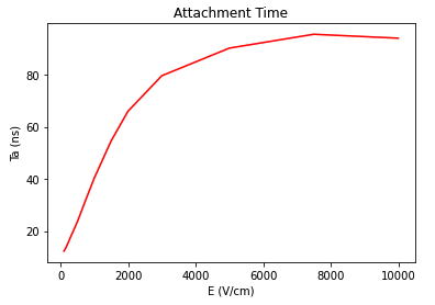
Calculating your attachment time with this (unchanged) driftvelocity and with the updated attachment coefficient I find something that looks rather good in agreement with the curves you showed (Boissonat, Hochhauser, Davies, …)
So my questions is rather how you computed your drift velocity … Did you make a gastable or did you extract it from your microscopic tracking simulation, and if yes, how did you do it?
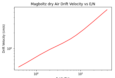
Going through the literature, the attachment of electrons on O2 in pure O2 and on O2 in Air (dry and humid) have been studied in literature since ~1960s [1-3], and these works are well known to the author of Magboltz, that has used them to model the cross-sections used as input and to validate afterwards the simulations, comparing to the experimental measurements. I found this interesting new article [4], and I compared the drift velocity of electrons in dry air computed with Magboltz to their measurements, and to me they look quite good: compare this figure to Fig 3 in the paper for 0% H2O:
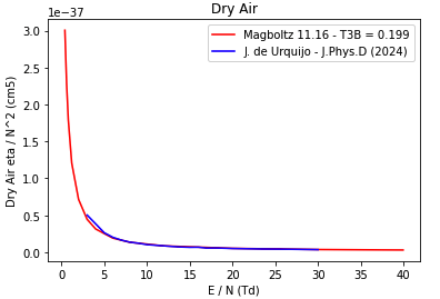
In this paper they also measured the 3-body attachment coefficient, normalized to the square of the gas density (eta/N^2) and aldo here magboltz (after modification with T3B = 0.199) gave good agreement:
So I would think that once the T3B parameter is correctly set, the attachment of electrons to O2 in dry air is in agreement with data, and I would assume it would be ok as well for humid air. Please let us know if you have still some unanswered questions. I’d like to read your thesis once it is finished ;-).
greets
Piet
[1] E. Kuffel (1959) Electron Attachment Coefficients in Oxygen, Dry Air, Humid Air and Water Vapour. Proc. Phys. Soc. 74 3.
[2] J.L. Moruzzi and D.A. Price (1973) Ionization, attachment and detachment in air and air-CO2 mixtures. J.Phys.D.: Appl. Phys 7 (1974) 1434-1440.
[3] T Taniguchi et al (1978) Three-body attachment in oxygen. J. Phys. D: Appl. Phys. 11 (1978) 2281.
[4] J. de Urquijo et al (2024) Two- and three-body attachment electron transport and ionisation in water-air mixtures, J.Phys.D: Appl Phys 57 (2024) 125205. Two- and three-body attachment, electron transport and ionisation in water-air mixtures - IOPscience
my code:
 import ROOT
import Garfield
import ctypes
import random
import math
import time
microscopic = True
gas = ROOT.Garfield.MediumMagboltz();
if microscopic:
    gas = ROOT.Garfield.MediumMagboltz("N2", 80.1, "O2", 19.9)
    # Dry Air N2:O2 80:20 - Load Cross Sections for Microscopic Tracking
else:
    gas.LoadGasFile("n2_80p1_o2_19p9_magboltz_modified.gas");
    # Dry Air N2:O2 80:20 - Load Gas File with Swarm Param for Avalance Monte-Carlo
gas.SetTemperature(273.15 + 20)
gas.SetPressure(760.)
# Thickness of the gas gap [cm] and voltage [V]
gap = .31
voltage = 1000.
# Make a component
cmp = ROOT.Garfield.ComponentConstant()
cmp.SetArea(0., -10., -10., gap, 10., 10.) # original
# cmp.SetArea(-gap, -10., -10., gap, 10., 10.) # heinrich
cmp.SetMedium(gas)
# field = voltage/gap
field = voltage/gap
print("Electric Field: ", field, "V/cm")
cmp.SetElectricField(field, 0., 0.)
# Make a sensor
sensor = ROOT.Garfield.Sensor()
sensor.AddComponent(cmp)
# declaration of c_type doubles
xe1 = ctypes.c_double()
ye1 = ctypes.c_double()
ze1 = ctypes.c_double()
te1 = ctypes.c_double()
ee1 = ctypes.c_double()
xe2 = ctypes.c_double()
ye2 = ctypes.c_double()
ze2 = ctypes.c_double()
te2 = ctypes.c_double()
ee2 = ctypes.c_double()
# and c_type ints
status = ctypes.c_int()
# Total number of electrons (nEvents or more if avalanche occurs)
nsumTOT = 0
# Total number of attached electrons
asumTOT = 0
nEvents = 1000
for i in range(nEvents):
    # Initial position and direction
    x0 = gap*random.random() # ROOT.RndmUniform()
    y0, z0, t0, e0, dx0, dy0, dz0 = 0., 0., 0., 0.1, 1., 0., 0.
    # number of electrons (1 or more if avalanche occurs)
    nsum = 0
    # number of attached electrons
    asum = 0
    # Avalanche class - - - Using Microscopic Tracking or Monte-Carlo
    if microscopic :
        aval = ROOT.Garfield.AvalancheMicroscopic()
        aval.SetSensor(sensor)
        aval.AvalancheElectron(x0, y0, z0, t0, e0, dx0, dy0, dz0)
    else :
        aval = ROOT.Garfield.AvalancheMC()
        aval.SetSensor(sensor)
        aval.AvalancheElectron(x0, y0, z0, t0, False)
    # Loop over the electron avalanches
    nsum = aval.GetNumberOfElectronEndpoints()
    for j in range(nsum):
        #AvalancheMicroscopic - 12 arguments | # AvalancheMC - 10 arguments - no arguments for energy of electron
        if microscopic :
            aval.GetElectronEndpoint(j, xe1, ye1, ze1, te1, ee1, xe2, ye2, ze2, te2, ee2, status)
        else :
            aval.GetElectronEndpoint(j, xe1, ye1, ze1, te1, xe2, ye2, ze2, te2, status)
        if (status.value == -7): asum = asum+1
    # end loop over nsum
    nsumTOT = nsumTOT + nsum
    asumTOT = asumTOT + asum
# end loop over nEvents
attachRatio = asumTOT*1.0/nsumTOT
freeRatio = 1 - attachRatio
# gas.PrintGas()
print("Number of events: ", nEvents)
print("Microscopic Tracking: ", microscopic)
print("Gap: ", gap, " [cm]")
print("Voltage: ", voltage, " [V]")
print("Field: ", field, " [V/cm]")
print("Total number of Electrons simulated", nsumTOT)
print("Total number of Attached electrons", asumTOT)
print("Ratio of free electrons: ", freeRatio)
print("Ratio of attach electrons: ", attachRatio)