Hi,
I’m having difficulties reproducing your results.
I used your SRIM files and your gas file but a slightly simplified geometry (parallel-plate chamber with a 1 cm gas gap). As you can see from first of the attached plots, the number of deposited electron/ion pairs increases with the pressure. There are some “steps”, because the number of electron/ion pairs has to be an integer. energydeposit.pdf (13.5 KB)
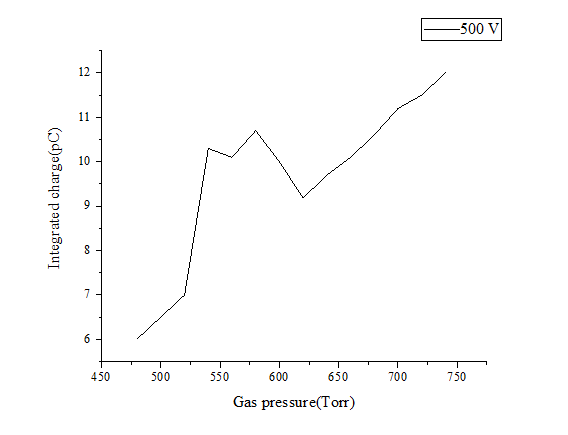
The second plot shows the integrated signal, with the contribution from the ions shown in red and the contribution from the electrons in orange. As you can see it also increases with increasing pressure. integratedsignal.pdf (13.6 KB)
Running these checks, I realised that by using TrackSrim and switching off energy fluctuations the average signal is a bit underestimated (because it’s “rounded off”/cut to the nearest integer) so that’s not ideal but the effect is not enormous.
Ok, I understand. So it looks like the problem with the geometry or the field map. When I use the Trim files, the number of deposited electron/ion pairs increases with the pressure too but a slice step that maybe caused by the integer of the plot too. But to the Srim files , I am so confused …would you please send me the minimal work files for me to compare?
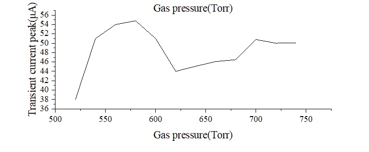
As what you said, the average electron/ion pairs increase with the pressure. And So is the integrated charge too. But as to the induced current , which is not proportional to the pressure since the change of the electron drift velocity. So maybe the plot I simulated using the Tracktrim maybe reasonable in the below, Is that right?
emm, I just want to use the equation I=nesv to calculate or simulate the v(electron drift velocity) value and find the relationship with the pressure and current. So is that unreasonable to use the peak current?
I’m not sure what the variables are in the equation you mentioned, but the program does indeed simulate the induced current using the drift velocity as function of the electric field, and the weighting field, using the Shockley-Ramo theorem.
My question was more if the peak current as function of pressure at constant electric field is a meaningful quantity. If you increase the pressure p but keep the electric field E the same, then there will be more charge deposited in the detector but the drift velocity will also change (because, to first order, it is a function of E/p).
Hi,
Thanks a lot for your reply and explanation.
I got stuck in the verification of the simulation results, such as the plot in the below, I don’t know why there are the mutations in the range from 540Torr to the 600Torr.
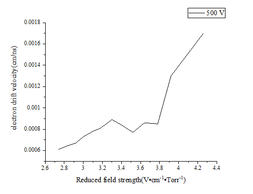
firstly I thought it must be the problem of the field map, then I considered it to be the wrong of the gas files or the EXYZ files. Finally I started to explain the reason. I remember the relationship between the electron drift velocity and reduced field strength is not proportional, something like the function
So I think maybe in the range from 540 to 600Torr the drift velocity has some situation. Then I use the simulation results to calculate the electron velocity according to the equation I=nev, n is for the electron numeber per cm, the e is the electron charge along the track . I got the curve like this in the below
We can find in the range from 540Torr to 600 Torr there indeed has a mutation area. According to the equation I=nev, Q=nevt, when the v is down, the Q is constant at the same condition, the parameter ne must increase. then we put the equation to this format Q=net f(E/p), when the ne increase, the Q must increase too. So when the E is constant at 500V(the whole data is simulated at the voltage of 500V), the Q will actually has the mutation area since the ne increase.
Hi,
Thanks a lot for your help and patient all these days
I have made a big progress in the Garfield++, next I will think about the voltage parameter
I remember you said that the “automatic calculation of the electron energy range in Magboltz seems to fail at 187.5 V/cm for this pressure and gas”,Is that problem solved now?
Besides ,do you have any advice about to analyze the relationship between the gas pressure , voltage, temperature, humidity with the electron charge or induced current.
OK, But there is a problem, I find that the calculation is from the minimal electric field to the maximum electric field. So if the electric field is from 179 to 1080, then it must have the 187.5 V/cm, then the simulation will be stopped .
I’m not sure I understand. You could, for instance, do something like this to cover the range of electric fields you are interested in with a reasonable number of intervals:
Ah, it’s a good idea, so that means the electric field value is 150, 170, 190,210…etc like this. right?
And besides, in the code gas.GenerateGasTable(ncoll); why the ncoll is set to 10?
You can reduce it a bit if you want. It means that Magboltz will 10×107 collisions at each electric field to calculate the drift velocity, diffusion coefficients etc.