I have simulated the average collected charge(the number of tracks simulated is 1000) in the gas ionization chamber caused by proton based on different gas pressure to find the optimization pressure value. Now there are few questions confused me a lot.
1, Why the integral charge value is so small about 6 to 7 fC.
2,the value of integral charge at the 700Torr and 640Torr is abnormal, which is bigger than the higher pressure.
3,how many tracks simulated would be reasonable, how to define them?

4, Why should we simulate the ion mobility? can we just delete them and just simulate the drift of the electron?
 // Load the ion mobility.
  auto installdir = std::getenv("GARFIELD_INSTALL");
  if (!installdir) {
    std::cerr << "GARFIELD_INSTALL variable not set.\n";
    return 1;
  }
  const std::string path = installdir;
  gas.LoadIonMobility(path + "/share/Garfield/Data/IonMobility_He+_He.txt");
I think @hschindl can help you.
I don’t understand the numbers on your plot. You say you have about 20 electron/ion pairs per track. That is not consistent with an average collected charge of 6 - 7 fC. And also the plots do not show a collected charge of 6 - 7 fC but orders of magnitude less. Maybe I miss something?
Also can you explain a bit better what is the purpose of your simulations? If fluctuations in the deposited charge are relevant for your than TrackTrim is a good choice. If you don’t care about fluctuations you might be better of using TrackSrim (like you did initially) and switch off straggling.
You don’t have to simulate the ion drift lines. But then you will miss part of the signal.
Hi,
Thanks a lot for your reply
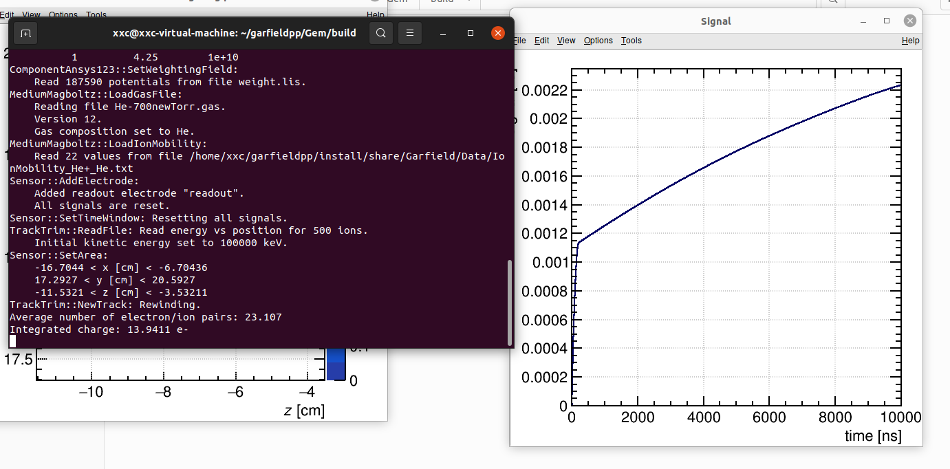
int the plot below , the last sentence of the terminal shows integrated charge:4.35249 E-, Does that mean the collected charge in total?
I assume to simulate the integral induced current or collected charge to find the optimization range of the gas pressure. Because I want the output signal is in the range I needed. So if the fluctuation is too abnormal , then I can’t get the a range of air pressure I wanted.

If this is a modified version of the program I sent you, then this number (integrated charge) corresponds to the last bin in the signal histogram (the plot on the right). So in your case it’s the collected charge after 500 ns. But as you can see from the plot, the integrated charge is still rising at this point; you need to wait longer if you want to capture the full deposited charge.
Having said that, if you are interested in the integrated charge after a long time and not in the signal as function of time, you don’t need to simulate the induced current at all, but just take the charge deposited by the track. And if you don’t care about fluctuations, you can just use SRIM.
I would also advise you to do some basic back of the envelope checks before running all these simulations, like what is the “active” thickness of your detector, what is the average energy loss of your particle over this distance, etc.
Hi,
Thanks a lot for your reply
you mean the integrated charge is just the charge in the last bin but not the whole charge in all bins?
I have just modified a little in the timebins, it seems reasonable in my program before when I set it as 500, apparent it is not suitable this time. I just need the integrated charge or the integrated induced current, either of them is ok. they are just used to represented to be a accumulated value at this gas pressure, if this value is bigger than I wanted, then I won’t choose this gas pressure when I do the actual experiment.
// Set the time bins for the induced current.
  const unsigned int nTimeBins = 500;
  const double tmin =  0.;
  // const double tmax = 2000.;
  const double tmax = 500.;
  const double tstep = (tmax - tmin) / nTimeBins;
  sensor.SetTimeWindow(tmin, tstep, nTimeBins);
The signal histogram initially contains the induced current. When you call IntegrateSignal(); the histogram is replaced by its integral. So when you retrieve the “signal” in the last bin after integrating, you get the charge accumulated over the entire time window. Please try to read the available documentation.
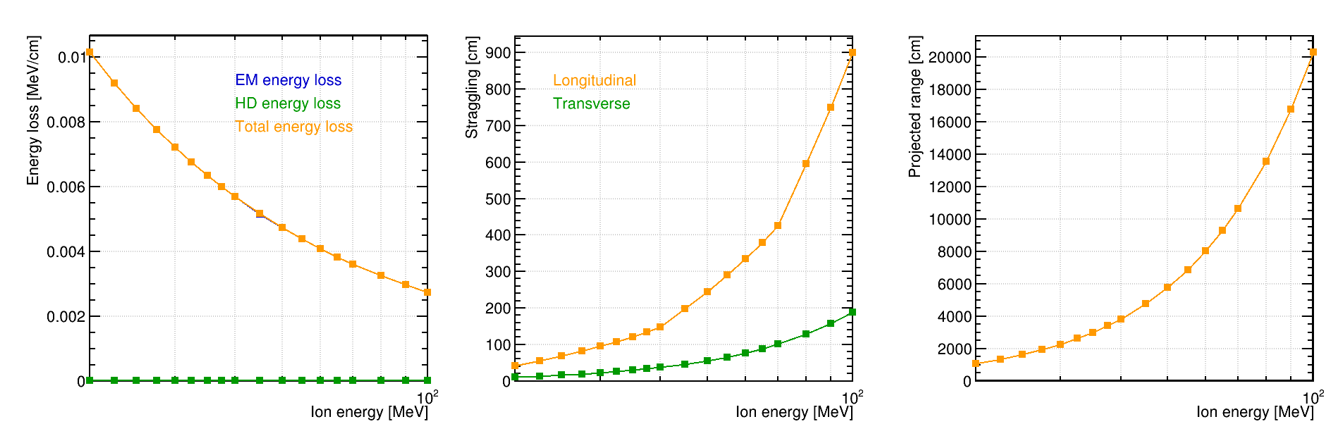
The top left plot shows the average energy loss per track length. Just look up the value at the projectile energy you are using.
Hi,
Thanks a lot for your reply and help
So can I interpret the result as an average value? And then I just multiply by 500 that I will get the charge accumulated over the entire time. Is that right?
If I want to get the value of induced current but not the integrate charged value. What should I do in the same condition(simulate hundred or thousand tracks once)
Yep, I know. If the proton’s energy is 100MeV, then the average loss per track length is approximately 0.00275 MeV/cm. However it is the energy deposited in the detector, what I wanted is the signal which is arriving at the electrode and collected. Are they the same?
Besides I want to find the result shows the range of the induced current between 0 and 160nA or the charge collected from 0 to 80pC。Then I can judge which gas pressure or voltage is better to chose.
No, if you call IntegrateSignals(); the histogram will contain the accumulated charge (in fC) as function of time. No need to multiply with anything.
Then don’t call IntegrateSignals();
Yes, if all electrons created by the particle eventually arrive at the electrode that you are reading out and if you are integrating over a long enough time.
Hi,
Thanks a lot for your patient explanation.
So the histogram of integratesignals mean the total value of the charge. I have deleted theIntegrateSignals(); the result turns to be this in the below
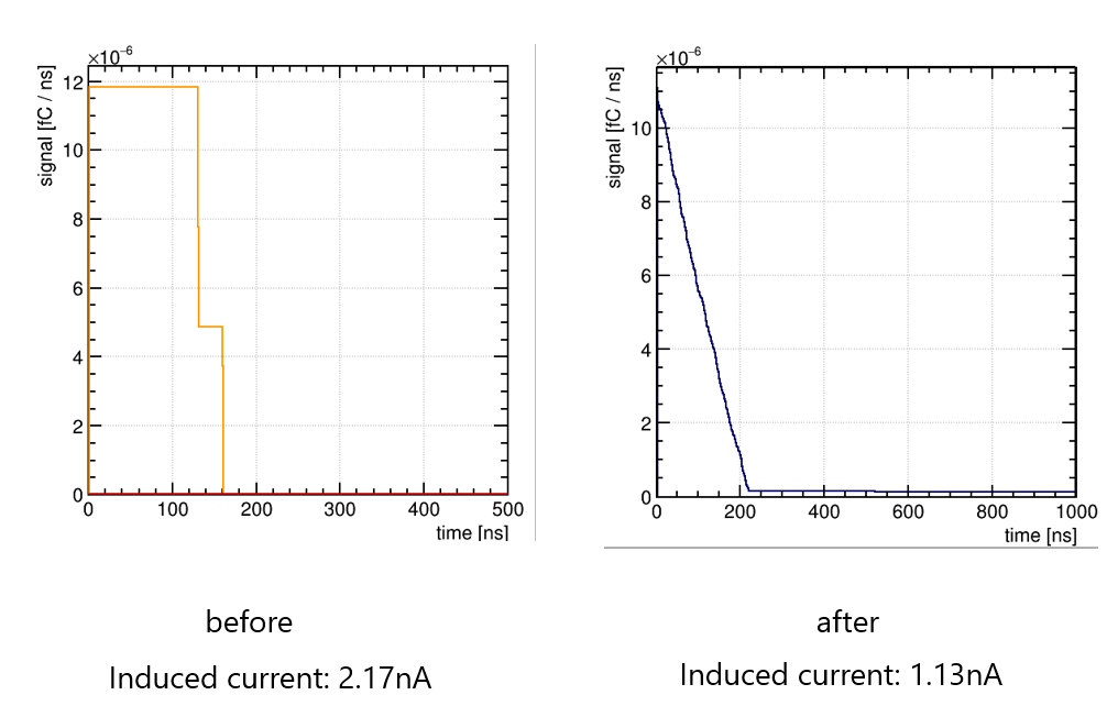
the left is the original code, the right is the modified code. I am a little confused that why the shape of the induced current signal will be changed? I have changed the gas file as you told me before, modifying the electric field point from 50 to 11, the logarithmic spacing to the linear spacing. what’s more , I have simulated more tracks (1000 proton once a time) but not one track. So that’s the reason for the shape changing. Also the accumulated induced current decreases after the code modified, why is that?
Hi,
There is still one question left I want to ask.
How can I get the integrated induced current by modifying the code, then I don’t need to calculate it through the plot by calculating the whole area of the entire curve.
By calling IntegrateSignals()!
Decreased with respect to what?
Ion drift is slow, if you want to catch the full ion signal you need to increase the time window. Or, as tried to suggest to you before, you just count how many electrons arrive at the electrode that you are reading out.
The total charge is not 13 fC but 13 electrons - which is very small.