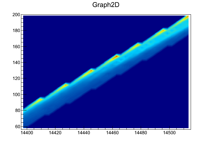
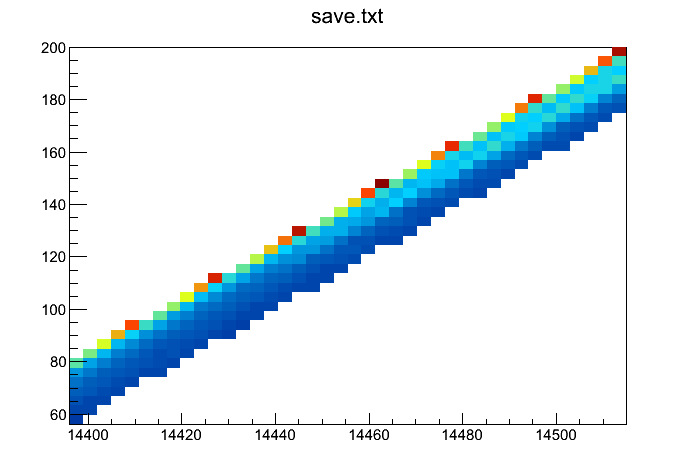
I am trying to plot the attached data (“save.txt”) using a TGraph2D graph and a 2D Contour plot.
As you may see at the attached figures, it looks that when i am using a ‘cont4’ option the graph is getting significantly distorted at the edges (the same happens when i use ‘surf’ options too); i assume that is related somehow to the way the contour regions are calculated.
When ‘cont5’ option is selected instead (or any Delaunay based option like ‘TRI’), things look good, but for presentation purposes i would prefer to have this tgraph2d with the ‘cont4’ option (in order to avoid these non-filled white areas within the contour region). Is this distortion upon cont4/surf option due to some bug, or is a limitation of the mathematical method used to calculate the contour regions?
many thanks for the tip. I see that this COL option approximates in a way what i want to do, however the limit on the pixel size ( even if i would increase the # of pixels to more than 500 from the source code) does not provide such a high quality figure as compared to the one that the cont4 option could provide.
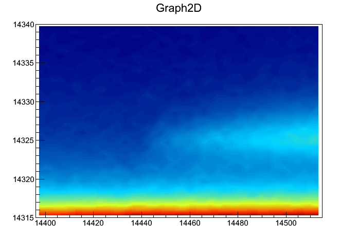
I would like to focus a bit more on the contour plot option problem instead (cont). I’ve tried a few more cases; To be more specific, when i am trying to plot the very same data in a different orientation (the data are attached as “save2.txt”) then the ‘cont4’ option is plotting the data correctly (the data are the same as the ones i provided at my first message; they are just rotated and translated on the xy plane). I do not know how useful observation that might be, but it shows in a way that the ‘cont4’ option does not treat the data in an isotropic way or something… is that behavior expected?
My point was to show that you should increase the number of bins of the underlying histogram. So set them to 200 along X an Y axis as I showed and use CONT4 if you want (instead of COL).
May be I should explain a bit more how these plots are produced. When you use histogram specific options like CONT4 or COL the plot produce is in fact coming from the underlying 2D histogram filled from the TGraph2D. The way this histogram is filled is the following:
For each bin we find which triangle is above the middle of the bin and fill the bin with the corresponding Z value. In your case you have a very sharp cut. If the bin are too big (which is the case when you are 40x40) the you may end up outside the sharp edge, because your edge is a diagonal in save.txt.
It is exactly like when you draw an oblique line and a horizontal line. With the oblique line you see the pixel and you don’t this the horizontal one.