Spiky log likelihood in Roofit

[fuji]

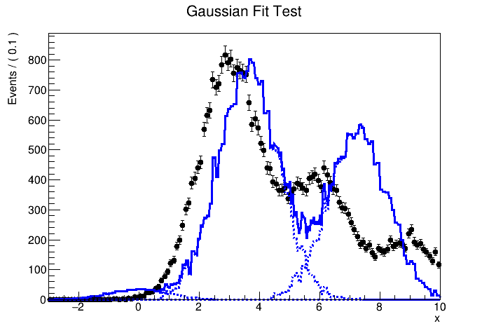
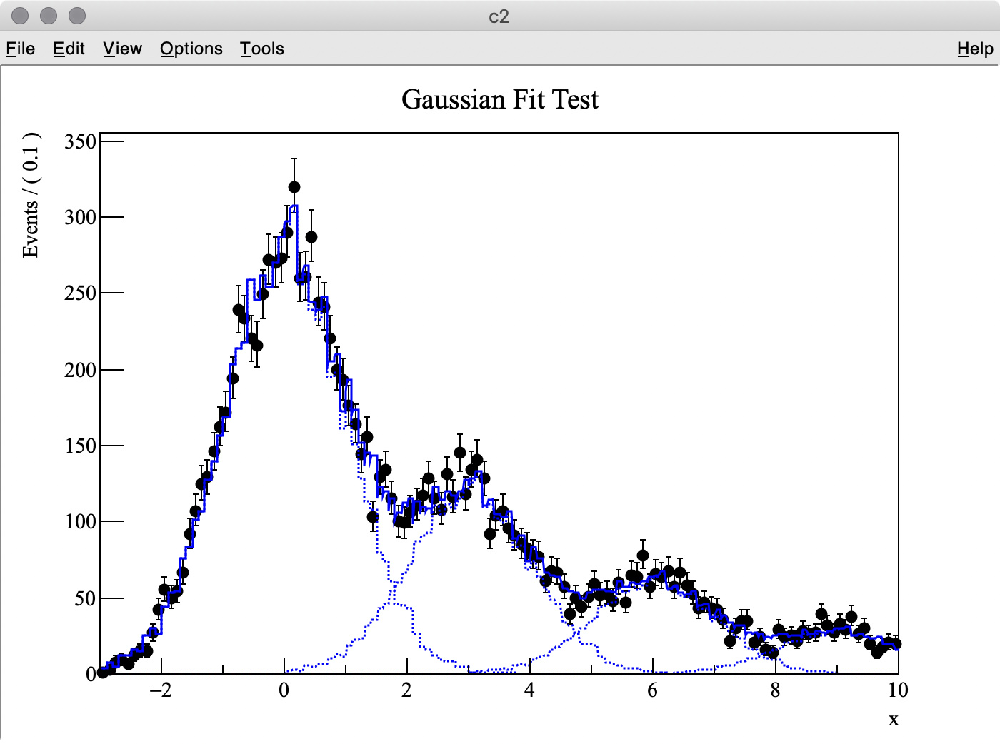
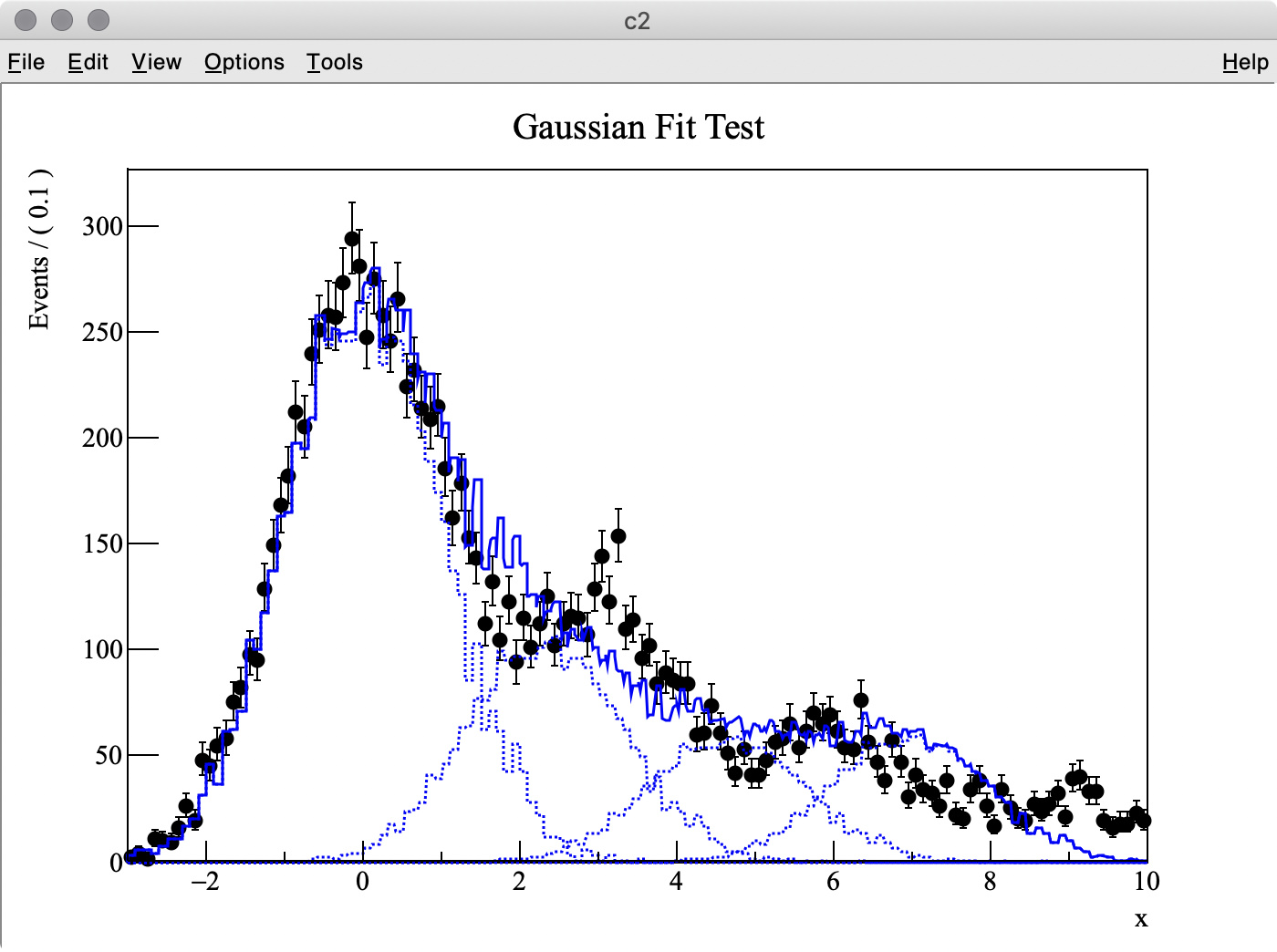
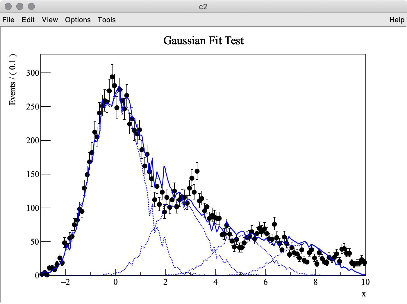
I try to fit simulation data (TH1 “h2”) containing three Gaussian peaks with a model probability distribution function (PDF) consisting of a sum of three Gaussian PDFs. The first Gaussian PDF is located at x = 0 (TH1 “h1”), the other two PDF shapes are identical with the first one, but they are horizontally shifted by dx and 2 * dx by using RooFormulaVar.

When making the model PDF, I set four parameters below :
dx : the x offset of shifted PDFs (2 * dx to be used for the second one)
p0, p1, p2 : scaling parameters for individual PDFs
pdf2.C (3.4 KB)

$ root
root [0] .x pdf2.C(1000000, 10000, 0.3)

The MC truth of dx is 3.0 but I often get very different best-fit values after minimization. This is probably because my PDF, which has a non-zero bin width, is shifted and sum of three binned PDFs is used.

The best fit values obtained for each parameter are listed below:

MIGRAD MINIMIZATION HAS CONVERGED.
FCN=-73640.4 FROM MIGRAD    STATUS=CONVERGED     264 CALLS         265 TOTAL
                    EDM=3.81233e-08    STRATEGY= 1  ERROR MATRIX UNCERTAINTY   0.0 per cent
 EXT PARAMETER                                   STEP         FIRST   
 NO.   NAME      VALUE            ERROR          SIZE      DERIVATIVE 
  1  dx           3.27545e+00   4.48015e-05   2.12661e-04   0.00000e+00
  2  p0           7.21953e+03   8.77706e+01  -1.02551e-03  -2.00881e-02
  3  p1           3.04091e+03   6.15363e+01  -6.97875e-04  -1.22533e-02
  4  p2           1.83955e+03   4.52509e+01   4.18298e-04  -1.22703e-02
                              ERR DEF= 0.5

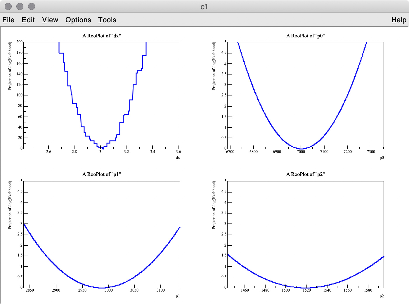
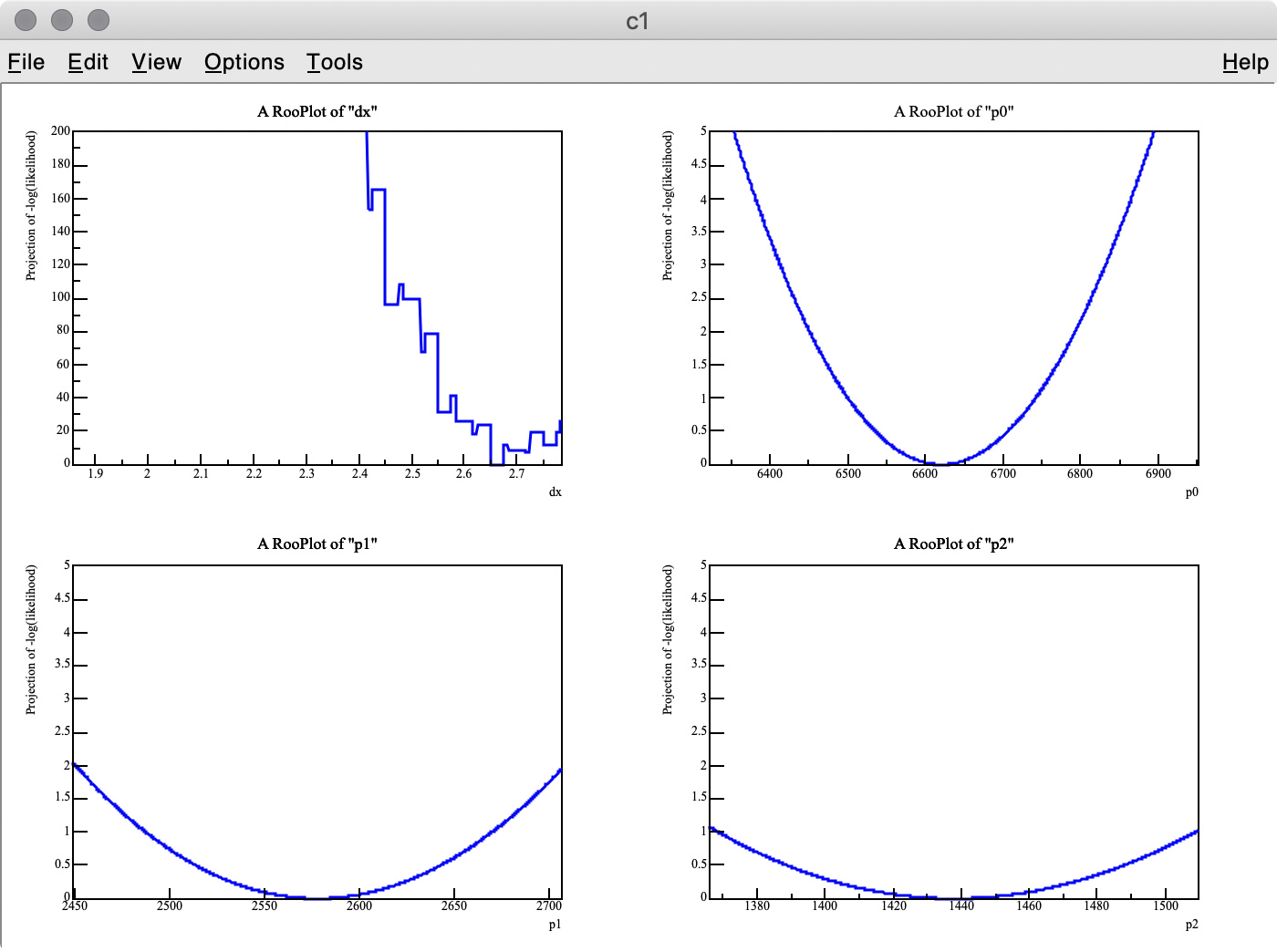
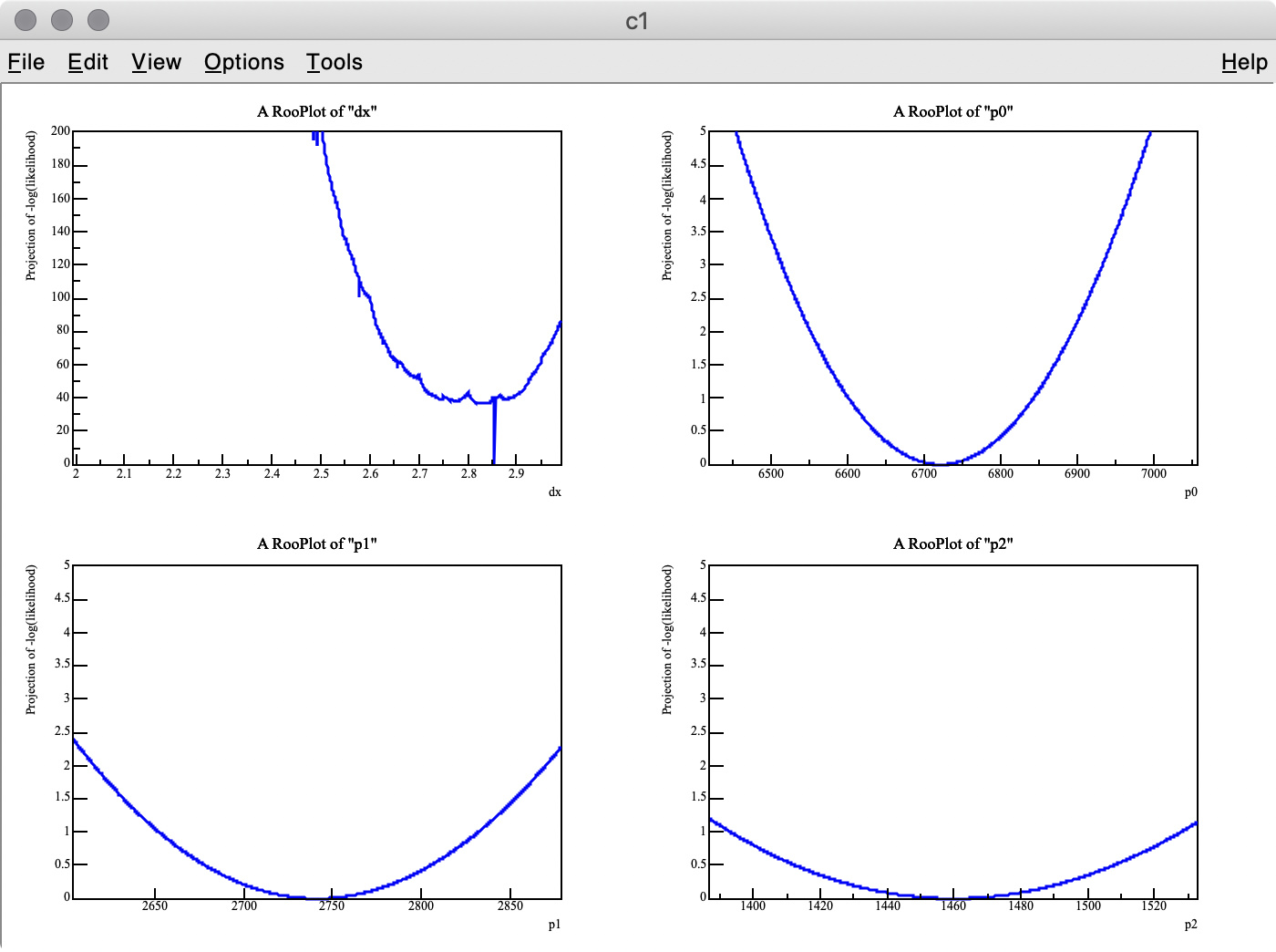
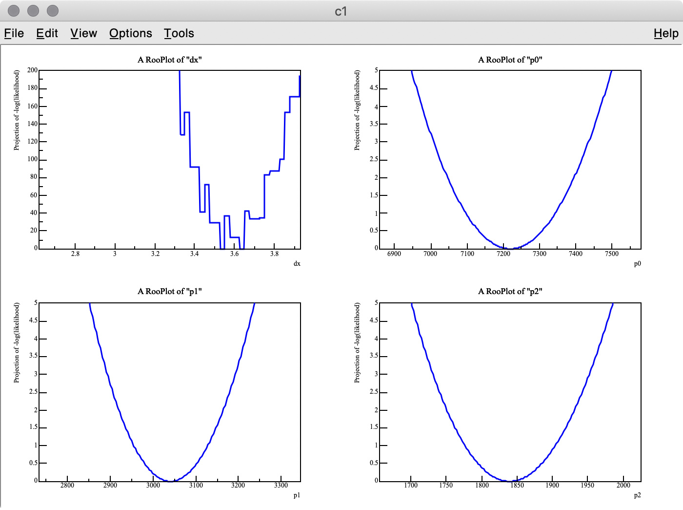
As you can see in the -log( likelihood ) of dx, it has spiky structure, resulting in wrong estimate of the best-fit value, whereas -log(likelihood) of p0, p1, and p2 are very smooth.

There are two points I am not certain about:

Q 1. Is there an easy way to find the best-fit dx value with the artificial peaks being ignored? I think a similar problem can happen when the energy scale of a MC PDF model is changed. I also tried to set the introder option to 1 to use interpolation, but it did not help much.

Q 2. I got 3.275 (MC truth = 3) as the best fit value of dx , but it looks like the minimum value of -log( likelihood ) of dx is around 3.6 in the top-left plot.
Why are these two values inconsitent?

[oshadura]

@StephanH can you help here please?

Cheers,
Oksana.

[StephanH]

Hello @fuji,

Is there a reason that you are not using proper Gaussian distributions? In my eyes, they would only have advantages:

• They are perfectly smooth.
• They are evaluated much faster.
• They can be integrated, shifted, scaled as necessary.

Further, I struggle to understand what you are trying to do. Are you trying to write down a model which is just
p1 * Gauss(x | mean1) + p2 * Gauss(x | mean2) + p3 * Gauss(x | mean3)?
Apparently, you also want that the three means are related to a single parameter.
If that’s the case, there is no need to fill three histograms for that. Just construct the model directly according to the formula above, and replace each mean by a RooFormulaVar that depends on the same parameter.

I also see that there is a coordinate transformation involved when constructing the RooDataHists. Unfortunately, I have no clue of how this works and what it is supposed to do. So if you could clarify a bit what the intention is, we can probably work something out.

[fuji]

Thank you @StephanH,

In my case, the actual PDF will not be a Gaussian but a non-Gaussian binned histogram made from the distribution of charge integration of oscilloscope waveforms. As shown in the attached plot, I would like to fit multi-peak charge distribution consisting of the pedestal (0 photoelectron, or 0 p.e.), 1 p.e., 2 p.e. and so on. The non-Gaussian model PDF is a bit different from a Gaussian because of the dark current of the photosensor we use.

The script I attached in my first post is for RooFit test purpose only as I am a beginner. I wanted to see if my fitting strategy works good at least in a simple simulation. That’s why I chose a Gaussian model distribution instead of using a real non-Gaussian distribution.

The plot shows a charge distribution made by integrating output waveforms from a silicon photomultiplier (SiPM). The leftmost peak corresponds to the pedestal (i.e., 0 p.e, no LED flash), which cannot be modeled with a simple Gaussian. As you can see, there is a discrepancy between the fit model (red solid) and data (black) at ~0.5 p.e… This is because the individual peaks are not Gaussian due to the long-tailed dark counts observed in the SiPM. My goal is to construct a non-Gaussian model PDF from the oscilloscope and the SiPM, and fit the data like this plot.

The shape of the 1 p.e. distribution is expected to be the same as that of pedestal because the SiPM gain is almost constant compared to the pedestal spread. That is the reason why I made a sum of a few x-shifted distributions to fit the data.

[StephanH]

Hey @fuji,

Ok, I get it. Maybe you want to try the
RooBukinPdf

It’s basically a Gaussian, but it allows for non-Gaussian tails on both sides. If something like this works, you can get around having to construct templates.
An advantage of an analytical function is that you can make them share parameters such as the tail or width parameters, and thus can make the model a bit more powerful.

If the Bukin doesn’t work, we can still try to figure out a template method.

[oxon]

Thank you again for the help. The model PDF that is made from SiPM dark-current waveforms cannot be modeled with the suggested function because its non-Gaussian components have a few other small peak structures due to 1-p.e., 2-p.e… dark-count events.

Of course we can first analytically fit the model PDF with existing functions to account for the all distribution characteristics, but our first motivation to use RooFits is to fit the charge distribution with another data histogram.

I think the main cause of this thread issue is that the fit error of dx is smaller than the data and model bin width, and thus -log(likelihood) can easily fall into a local minimum (local artificial spike). Is there any way to force MIGRAD to have a user-specified fixed step-size value? If we keep it to the bin width, I think the issue can be resolved.

Another possible solution is to smoothly divide the individual bin contents when dx is not a multiple of the bin width. But I could not find a such functionality in RooFit. Is it possible?

[StephanH]

I don’t immediately see a way to do this.

I guess that you are right that the spikes in the likelihood result from jumping from one bin to the other. One possible solution is to use more bins and interpolate between them. What happens if you run the fit with interpolation > 0?

[StephanH]

I ran the example. It looks like the fit model doesn’t have enough flexibility to capture the data.

The spacing and the mean values of the distributions seem to be wrong, so there’s now way to get the fit right. Some ideas:

• Can it be that the spacing and normalisation are too much hard coded?
• Wouldn’t it be better if the fit could actually vary the distance between the peaks?
• The templates might also be too noisy because of statistical fluctuations. For some reason, interpolation doesn’t do much for me, but the Barlow-Beeston method can take uncertainties of the templates into account.
  See here for details: https://root.cern.ch/doc/master/rf709__BarlowBeeston_8C.html

[oxon]

I found a mistake in our sample script pdf2.C in which the peak at the rightmost was missing in the model. Fixing this stupid mistake, the fit result became better. But sometimes we see similar artificial spikes and local minima.

The attached is a modified version of the script.
pdf2.C (3.6 KB)

root [0] .x pdf2.C(10000, 10000, 0.3, 1, 0)
where 1 is the random seed, and 0 is int_order for interpolation. The result is not very bad.

But if I set another random seed, 3, I get a bad result.
root [1] .x pdf2.C(10000, 10000, 0.3, 3, 1)

With the interpolation option being on, an artificial spike appears.
root [1] .x pdf2.C(10000, 10000, 0.3, 3, 1)

I will try the BB method to take into account the model fluctuation. However, I suppose that artificial spikes can appear again when the horizontal position of the model 1D histogram is changed even with the BB method. I would appreciate it you could suggest an idea to get rid of spikes in -log(likelihood).

Using the BB method in our case will introduce another issue that the model histogram fluctuation is counted multiple times independently, resulting in an overestimate of model fluctuation. But I will try to find a way to avoid this issue. It is probably beyond the scope of the ROOT forum.