Dear Garfield experts,
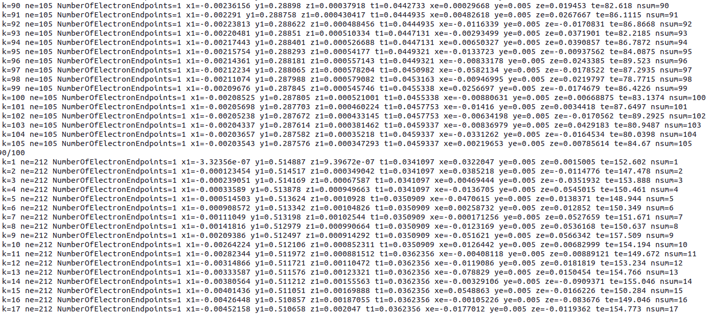
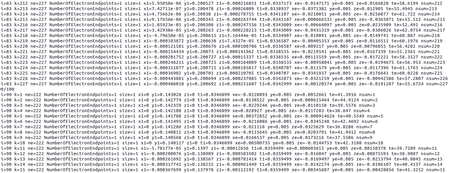
I am using the fe55.C example modified in order to simulate the response of a micromegas detector on a point Fe55 iron X-ray source. Then I track the electrons from the photon absorption and calculate the deposited charge on the mesh using the RKF method at first.
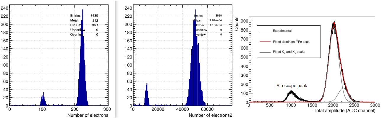
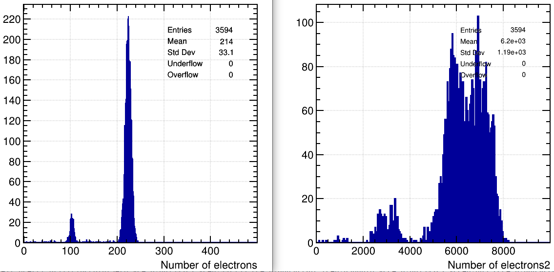
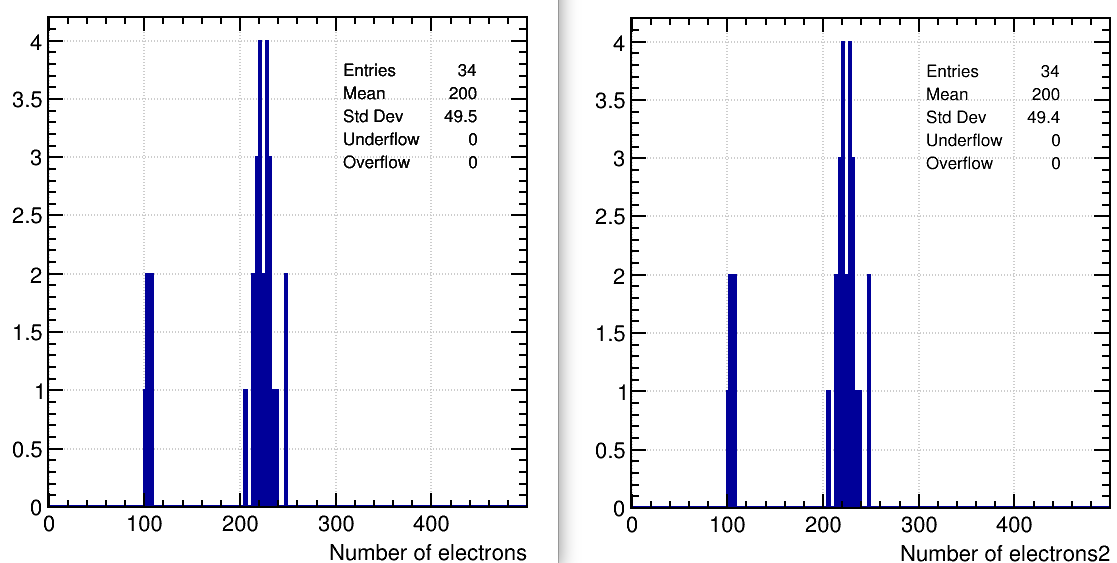
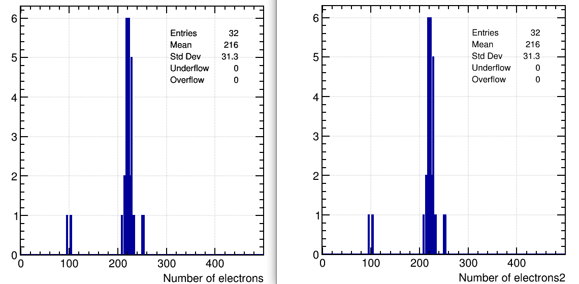
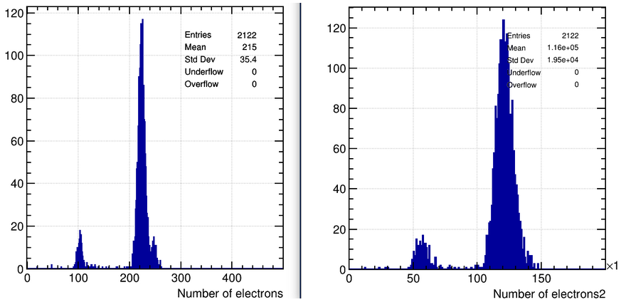
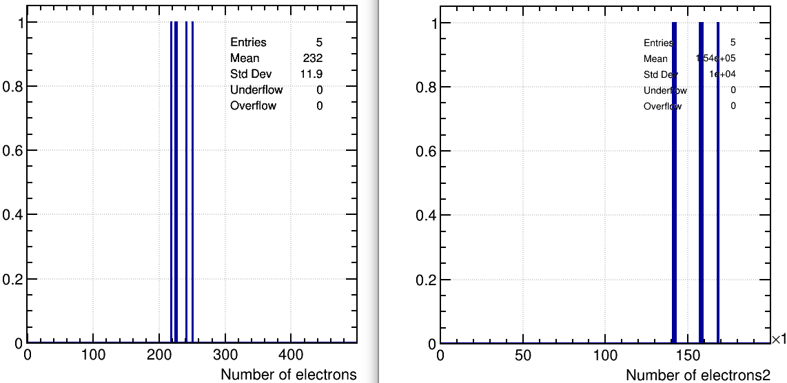
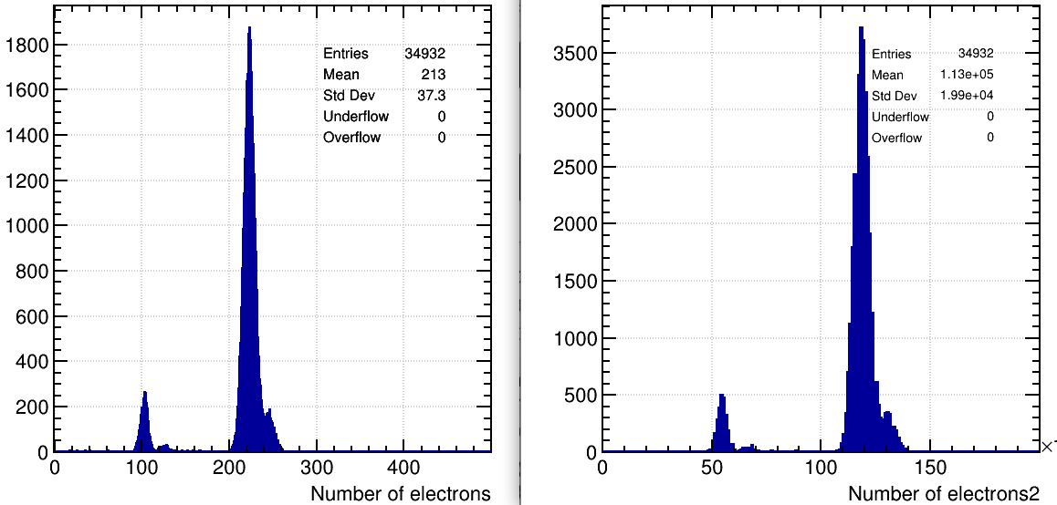
In the left picture (number of electrons) are the electrons produced which seems to be in the right relative position concerning the Argon escape peak and the Iron dominant peak.
In the middle picture (number of electrons 2), where the number of electrons is shown on the mesh, why the argon (??) peak is placed too far from the dominant one?
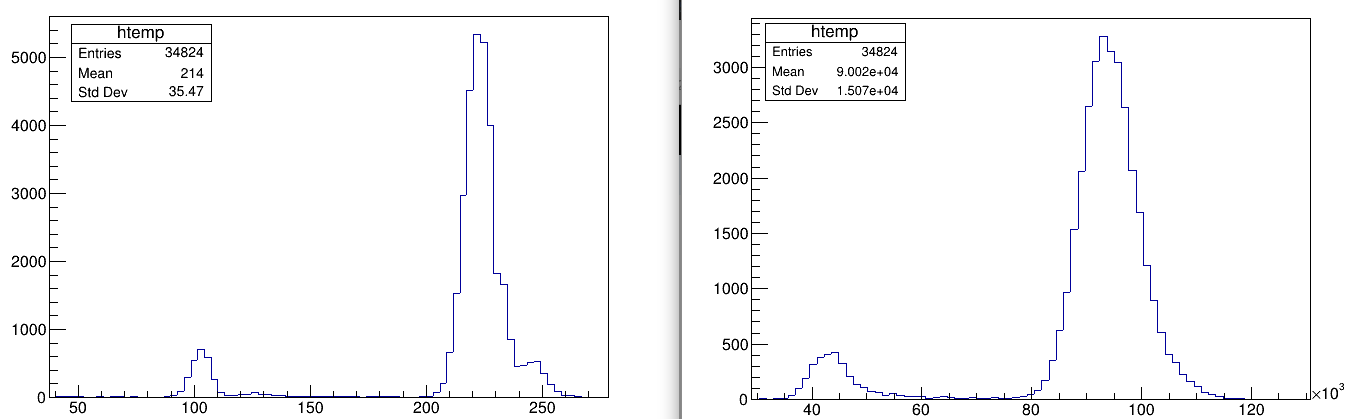
The third picture on the right is the experimental one that we would like to simulate…
Any suggestion??
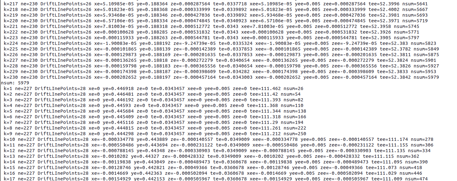
The code I used:
// X-ray conversion
// -------------------------------------------------------------------
// Simulate the Fe55 spectrum
//
// Thanks to Dorothea Pfeiffer and Heinrich Schindler from CERN for their help.
// -------------------------------------------------------------------
// Lucian Scharenberg
// scharenberg@physik.uni-bonn.de
// 05 APR 2018


#include <iostream>
#include <fstream>
#include <cmath>

#include <TCanvas.h>
#include <TROOT.h>
#include <TApplication.h>
#include <TH1F.h>

#include "Garfield/TrackHeed.hh"
#include "Garfield/MediumMagboltz.hh"
#include "Garfield/SolidTube.hh"
#include "Garfield/GeometrySimple.hh"
#include "Garfield/ComponentConstant.hh"
#include "Garfield/Sensor.hh"
#include "Garfield/FundamentalConstants.hh"
#include "Garfield/Random.hh"
#include "Garfield/Plotting.hh"
#include "Garfield/ComponentAnalyticField.hh"

#include "Garfield/ViewDrift.hh"
#include "Garfield/DriftLineRKF.hh"

#include "Garfield/AvalancheMicroscopic.hh"

using namespace Garfield;

int main(int argc, char * argv[]) {

  TApplication app("app", &argc, argv);
  plottingEngine.SetDefaultStyle();


  MediumMagboltz gas;
  gas.LoadGasFile("Ar95_iso5_1atm.gas");


   // Build the Micromegas geometry.
  // We use separate components for drift and amplification regions.

  // 50 um amplification gap.
  ComponentAnalyticField cmpA;
  cmpA.SetMedium(&gas);
  constexpr double yMesh = 0.005;
  constexpr double vMesh = 0.;
  constexpr double vPad = 350.;
  cmpA.AddPlaneY(yMesh, vMesh, "mesh1");
  cmpA.AddPlaneY(0., vPad, "pad");
  cmpA.AddReadout("mesh1");
  cmpA.AddReadout("pad");
  // 10 mm drift gap.
  ComponentAnalyticField cmpD;
  cmpD.SetMedium(&gas);
  constexpr double yDrift = yMesh + 1.0;
  constexpr double vDrift = -600.;
  cmpD.AddPlaneY(yDrift, vDrift, "drift");
  cmpD.AddPlaneY(yMesh, vMesh, "mesh2");
  cmpD.AddReadout("mesh2");
  cmpD.AddReadout("drift");
  // Assemble a sensor.
  Sensor sensor;
  sensor.AddComponent(&cmpA);
  sensor.AddComponent(&cmpD);
  sensor.SetArea(-5.0, 0., -5.0, 5.0, yDrift, 5.0);

  sensor.AddElectrode(&cmpA, "mesh1");
  sensor.AddElectrode(&cmpA, "pad");
  sensor.AddElectrode(&cmpD, "mesh2");
  sensor.AddElectrode(&cmpD, "drift");


   // RKF integration.
  DriftLineRKF drift;
  drift.SetSensor(&sensor);


  // Use Heed for simulating the photon absorption.
  TrackHeed track(&sensor);
  track.EnableElectricField();
  // Histogram
  const int nBins = 500;
  TH1::StatOverflows(true);
  TH1F hElectrons("hElectrons", ";Number of electrons;",
                  nBins, -0.5, nBins - 0.5);

  TH1F hElectrons2("hElectrons2", ";Number of electrons2;",
                  200, -0.5, 80000 - 0.5);


  const unsigned int nEvents = 10000;

	  for (unsigned int i = 0; i < nEvents; ++i) {
   		 if (i % 1000 == 0) std::cout << i << "/" << nEvents << "\n";
    // Initial coordinates of the photon.

    int nsum = 0;
    int ne = 0;

    const double x0 = 0.;
    const double y0 = 1.0;
    const double z0 = 0.;
    const double t0 = 0.;

    const double egamma = 5900;

    track.TransportPhoton(x0, y0, z0, t0, egamma, 0., -1.0, 0., ne);

    	if (ne > 0) hElectrons.Fill(ne);

		for (int k = 0; k < ne; ++k) {


      nsum += ne;


  double xe = 0., ye = 0., ze = 0., te = 0., ee = 0.;
  double dx = 0., dy = 0., dz = 0.;
  track.GetElectron(k, xe, ye, ze, te, ee, dx, dy, dz);


  drift.DriftElectron(xe, ye, ze, te);


      double xee = 0., yee = 0., zee = 0., tee = 0.;
      int status = 0;
      drift.GetEndPoint(xee, yee, zee, tee, status);
      yee = yMesh - 1.e-10;
      drift.DriftElectron(xee, yee, zee, tee);

std::cout << "k=" << k+1 << " ne=" << ne << " xe=" << xe << " ye=" << ye << " ze=" << ze << " te=" << te << " xee=" << xee << " yee=" << yee << " zee=" << zee << " tee=" << tee << " nsum=" << nsum <<"\n";
}

    if (nsum > 0)     hElectrons2.Fill(nsum);

 	if (nsum > 0)      std::cout << "nsum: " << nsum << "\n";

  }

  TCanvas c("c", "", 600, 600);
  c.cd();
  hElectrons.SetFillColor(kBlue + 2);
  hElectrons.SetLineColor(kBlue + 2);
  hElectrons.Draw();
   c.Update();


   TCanvas c2("c2", "", 600, 600);
  c2.cd();
  hElectrons2.SetFillColor(kBlue + 2);
  hElectrons2.SetLineColor(kBlue + 2);
  hElectrons2.Draw();


  c2.Update();
  app.Run(true);
}