Addition of oxygen with not substantial effect on a 2 ll plate detector

[gtsileda]

Dear experts,

As a continuation of the topic discussed in Simulation of Fe55 source on a parallel plate detector
a 2 parallel plate detector is built operated with Ar-Isobutane (95/5)% (simplified geometry for a micromegas detector).

fe55.C (5.0 KB)
gasfile.cpp (1.6 KB)
ArIso5_1pcO2.txt (67.3 KB)
ArIso5new.txt (61.9 KB)
I upload the gas files used (in txt extension), the program used for the production of the gas files as well as the program for evaluating the simulation for 1000 events using a Fe55 source.
The picture attached shows the results concerning the electrons from ionization that arrive at the mesh (1st end of the 2 // plate detector) and the electrons at the pad (2nd end). There is only ~ 10% drop of the gain in the main Fe55 peak while at the end of the drift there is no such effect…
I expected a much higher gain drop due to attachment and an obvious contribution at the gain at the end of the drift…
I wonder whether you could have a look and let me know your always valuable remarks…

Thanks a lot in advance

Best regards

Georgios
Processing: fe55.C…
Processing: gasfile.cpp…

[devajith]

Hi @gtsileda,

Adding @hschindl in the loop.

Cheers,
Dev

[hschindl]

Hi,
sorry for the late reply! Can you do a couple of checks?

• What is the value of the attachment coefficient at the electric field in the drift gap? And what is the corresponding probability of losing an electron to attachment?
• What are the values of the attachment coefficient and Townsend coefficient in the avalanche gap?

[gtsileda]

Dear expert,

I have not fully understand how to extract those values…
The drift field is from -300 → 0 V at 1 cm and the avalance 0 → +320 V at 0.005 cm.
Thus, in drift → att ~ 2.5 [1/cm] and in avalance → att ~ 0.5 [1/cm].
Is it reasonable?

Thanks a lot in advance

Georgios

[hschindl]

Hi Georgios,

to retrieve the electric field in the drift gap, you can do something like this

auto edrift = cmpD.ElectricField(0., 0.5 * (yMesh + yDrift), 0.);

(but you can of course also simply calculate it yourself). Then to retrieve the attachment coefficient at this field, you can do something like this

double eta = 0.;
gas.ElectronAttachment(edrift[0], edrift[1], edrift[2], 0., 0., 0., eta);

[gtsileda]

Hi Heinrich,

Thanks for the tips. I did what you suggested and more or less I got the values as stated in my previous post just visually from the plots.
I did the following:

std::cout << “\nField intensity in the middle of drift region:\n”;
double y1 = 0.5 * (yMesh + yDrift);
auto edrift = cmpD.ElectricField(0., y1, 0.);
//auto edrift = cmpD.ElectricField(0., 0.5 * (yMesh + yDrift), 0.);

double magnitude1 = sqrt(edrift[0] * edrift[0] + edrift[1] * edrift[1]);
std::cout << “At y = " << y1 << " cm:\n”;
std::cout << " E = " << magnitude1/1000 << " kV/cm\n";

double eta1 = 0.;
gas.ElectronAttachment(edrift[0], edrift[1], edrift[2], 0., 0., 0., eta1);

std::cout << eta1 << “\n”;

///////////////////////////////////////////////////
std::cout << “\nField intensity in the middle of avalanche region:\n”;
double y2 = 0.5 * (yMesh);
auto edrift2 = cmpA.ElectricField(0., y2, 0.);

double magnitude2 = sqrt(edrift2[0] * edrift2[0] + edrift2[1] * edrift2[1]);
std::cout << “At y2 = " << y2 << " cm:\n”;
std::cout << " E = " << magnitude2/1000 << " kV/cm\n";

double eta2 = 0.;
gas.ElectronAttachment(edrift2[0], edrift2[1], edrift2[2], 0., 0., 0., eta2);

std::cout << eta2 << “\n”;

I am getting:

Field intensity in the middle of drift region:
At y = 0.505 cm:
E = 0.3 kV/cm
2.45549

Field intensity in the middle of avalanche region:
At y2 = 0.0025 cm:
E = 64 kV/cm
0.406007

If this is correct, how it explains those results?

Best regards

Georgios

[hschindl]

Ok, good! What fraction of the primary electrons to you expect to be lost due to attachment based on the value of eta in the drift region?

[gtsileda]

@hschindl

What fraction of the primary electrons to you expect to be lost due to attachment based on the value of eta in the drift region?

If I am not mistaken, the exponential decay law for electron survival in the presence of attachment
in this case gives: e^(n*d) where n = 2.46cm^(-1) and d=1 cm. Thus, subtracting it by 1 provides the fraction of electrons lost due to attachment which is ~ 91%. It seems that only ~ 9% of the electrons would survive the full 1 cm drift in this field condition. If this is true, why the amplitude spectra as given in the pict of the 1st post does not change significantly with the presence of 1% O2 compared to the initial Ar-isobutane mixture?

[Piet]

Dear Georgios

Indeed, what you get this way is exactly what you read from plots that you made that are in my opinion reasonable. What I do not understand is what exactly you do not understand from your original results (at least for the lefthand plots).

It is not completely clear from your attached fe55.C file where you fill the histograms you show, because I see the fill functions commented out:

track.TransportPhoton(x0, y0, z0, t0, egamma, 0., -1.0, 0., ne);
// Fill number of electrons in ionization
// if (ne > 0) hElectrons.Fill(ne);

and

// Fill number of electrons at the pad
//if (nsum > 0) hElectrons2.Fill(nsum);

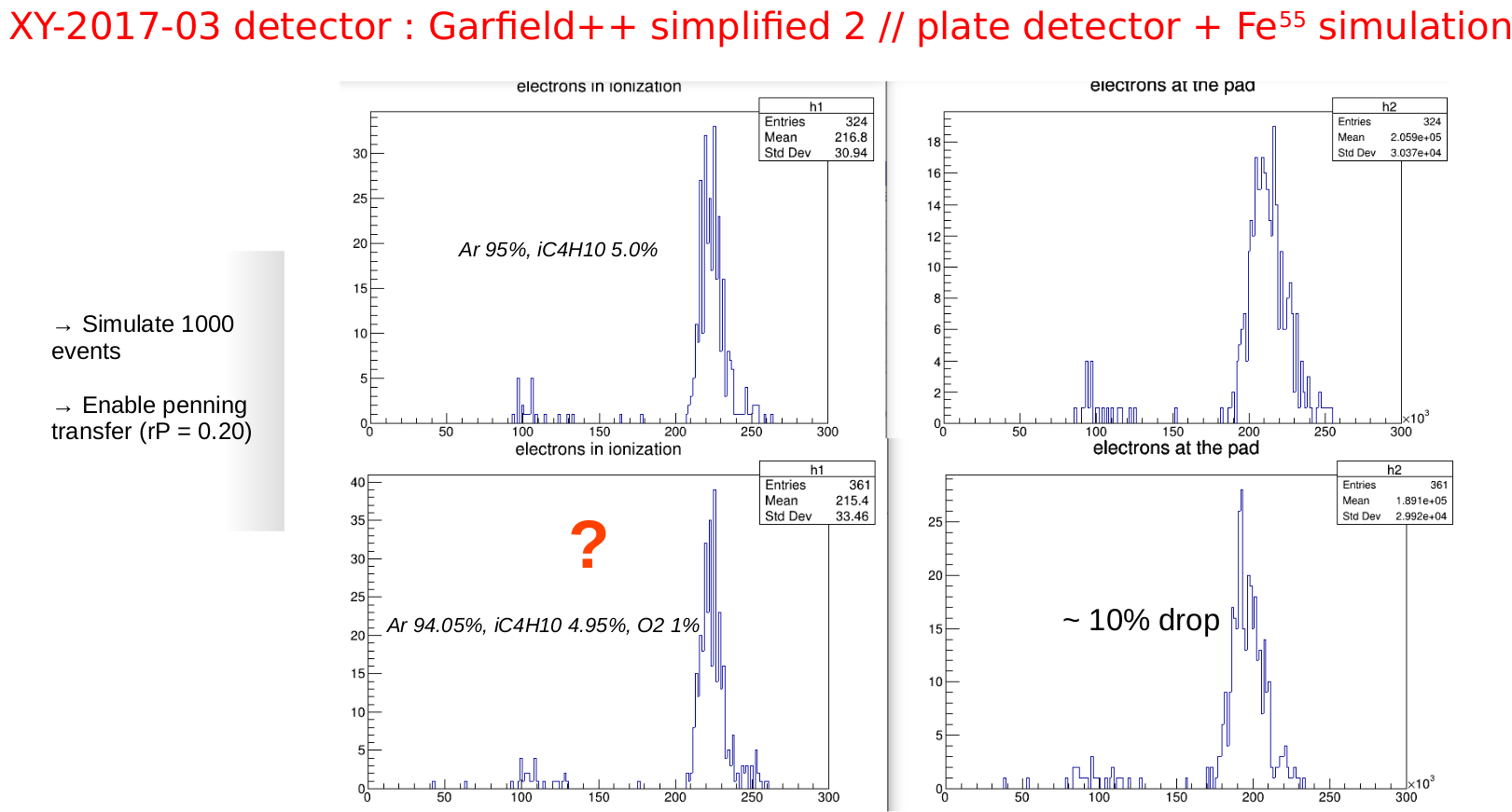
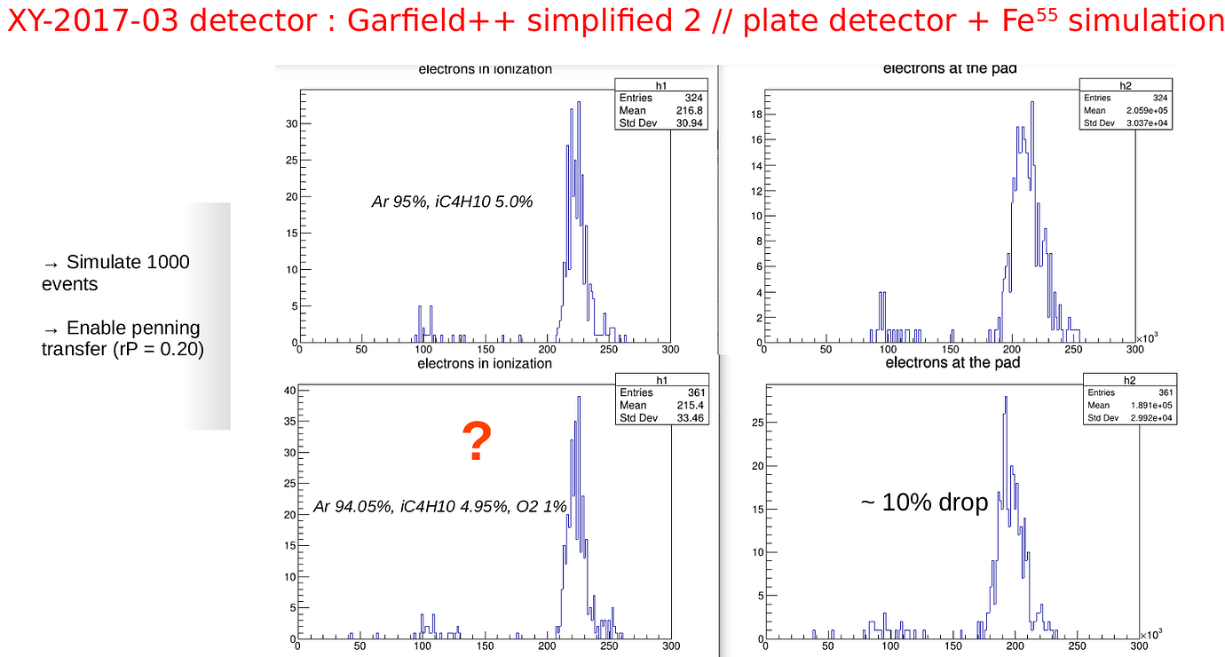
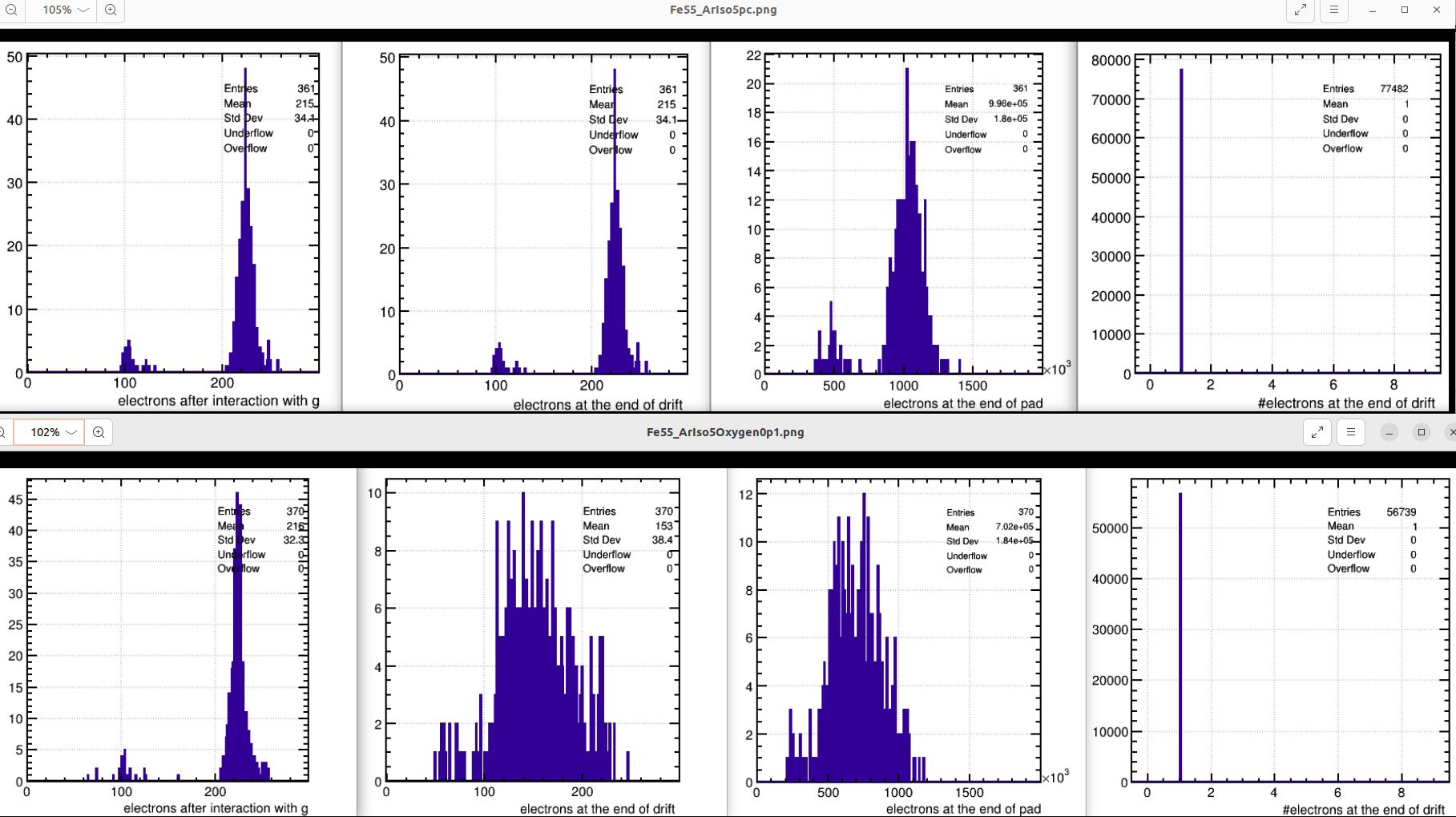
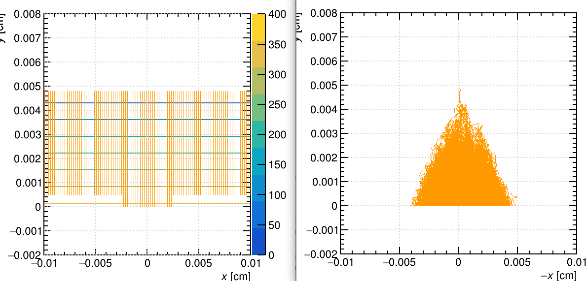
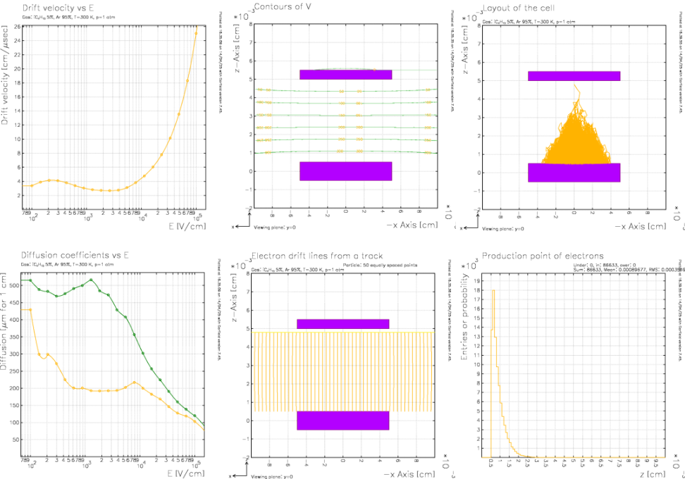
Let me for now presume these are the positions in your code that you filled those histograms. Then in this case the results (your plots) look perfectly reasonable. The leftmost plot is not the amount of electrons at the end of the drift, but is the amount of electrons directly after the interaction of the photon in the gas, calculated with heed. this is before any attachment can happen, because you are not yet simulating the transport of the ionization electrons in the gas. So it is perfectly reasonable that top and bottom plot have the same value (~215 electrons). Instead the right hand plots you fill at the end of your amplification volume and indeed you see a 10% drop, that likely is mostly due to the drift in the 1cm driftgap and not so much due to attachment in the avalanche region. If you would like to know how many electrons arrived at the end of the drift region, you should create another plot and fill the number of electrons obtained at the end of the AvalancheElectron calculation done in the driftfield:

int n_mesh = driftD.GetNumberOfElectronEndpoints();
if(n_mesh > 0) hElectrons1.Fill(n_mesh);

However, in the way you program, I believe there is something that might not be completely correct. Immagine that you drift an electron in the driftgap from position and time (x1, y1, z1, t1), but it gets attached at a certain time at a certain position (x2,y2,z2,t2). When you call the function

driftD.GetElectronEndpoint(k2, x1, y1, z1, t1, e1, x2, y2, z2, t2, e2, status);

it will get you back exactly the position (x2,y2,z2,t2) as endpoint of this electron, which is not on the boundary between the drift and the amplification volume. Instead you proceed with:

driftA.AvalancheElectron(x2, yMesh - 1e-10, z2, t2, 0, 0, 0, 0);

which means that for you it is not lost, and you place this electron in the amplification volume at same x2,z2 and at time t2, but with now with y-value such that it is inside and you run the avalanche again. This to me explains why you have always the same number of entries in histograms h1 and h2. So this in my opinion you should do in a different way (e.g. check whether the y2 value is close enough to the boundary of your driftgap).

The only thing I am a bit puzzled about is why apparently you do not have any multiplication in your amplification region. Apparently your nsum is always equal to n_mesh, which is equal to ne as explained earlier). So this you should try to find out a bit, maybe adding some couts of your driftA.GetNumberOfElectronEndpoints and/or also using the function driftA.GetAvalancheSize (neA, niA).

greets
Piet