Signal calculation of low energy particles and fission fragments in a Micromegas geometry

Hello! I want to retrieve the signal of low energy ions and fission fragments (in the script I am attaching below,I want to track α-particles with kinetic energy of 5 MeV) passing through a Micromegas geometry.The code I am using is a combination of asacusa,DriftTube,SRIM and other examples.Retrieving the outputs Ι am attaching after the code,I had the following questions:

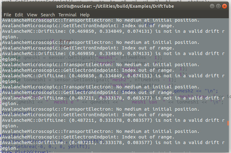
  1. I see that,in most examples,functions DriftLineRKF,AvalancheMicroscopic,AvalancheMC are being used for signal calculation.In my script,I am using only DriftLineRKF as you can see. I want to know if this is the most efficient (or even a correct!) way to retrieve the signal or should I use a combination of AvalancheMicroscopic,AvalancheMC and DriftLineRKF?

  2. What exactly is the definition of dx,dz,dz in TrackSrim::NewTrack?.Firstly I thought it was just a definition of direction using a beginning (x0,y0,z0) and an ending point (dx0,dy0,dz0) of the track but I noticed that maybe I misunderstood.Are they related to the angles? Can you make it clear to me?

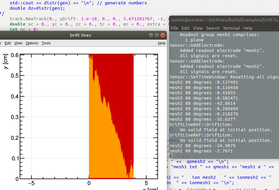
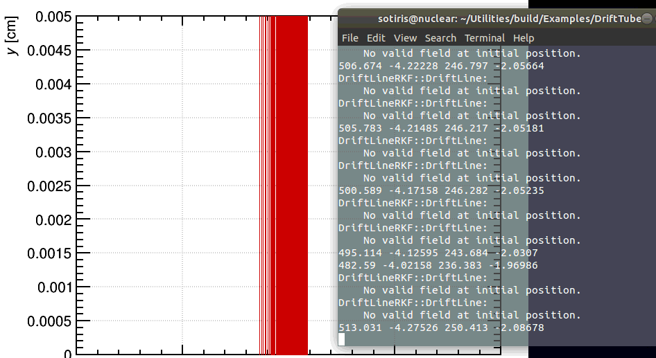
  3. Using DriftLineRKF::GetElectronSignal,I am always getting 0.Could you tell me what am I missing here? Also,I am wondering why the total signal on mesh2 is positive,even though the electrons are being collected there.Is it maybe due to the large number of positive ions in amplification region and so the total signal is positive?

  4. Is the usage of DriftLineRKF::SetElectronSignalScalingFactor(nc) correct in the code (Ln 149) or should this be in/out of the loop?

Any answer to these or any suggestion/correction on the code would be Really helpful.

#include <iostream>
#include <fstream>
#include <cstdlib>
#include <cmath>

#include <TCanvas.h>
#include <TROOT.h>
#include <TApplication.h>				

#include "Garfield/ViewCell.hh"
#include "Garfield/ViewDrift.hh"
#include "Garfield/ViewSignal.hh"

#include "Garfield/ComponentAnalyticField.hh"
#include "Garfield/MediumMagboltz.hh"
#include "Garfield/Sensor.hh"
#include "Garfield/DriftLineRKF.hh"
#include "Garfield/TrackHeed.hh"
#include "Garfield/TrackSrim.hh"

using namespace std;
using namespace Garfield;

bool readTransferFunction(Sensor& sensor) {

  std::ifstream infile;
  infile.open("mdt_elx_delta.txt", std::ios::in);
  if (!infile) {
    std::cerr << "Could not read delta response function.\n";
    return false;
  }
  std::vector<double> times;
  std::vector<double> values;
  while (!infile.eof()) {
    double t = 0., f = 0.;
    infile >> t >> f;
    if (infile.eof() || infile.fail()) break;
    times.push_back(1.e3 * t);
    values.push_back(f);
  }
  infile.close();
  sensor.SetTransferFunction(times, values);
  return true;
}

int main(int argc, char * argv[]) {

  TApplication app("app", &argc, argv);

  // Set the gas mixture.

  MediumMagboltz gas;
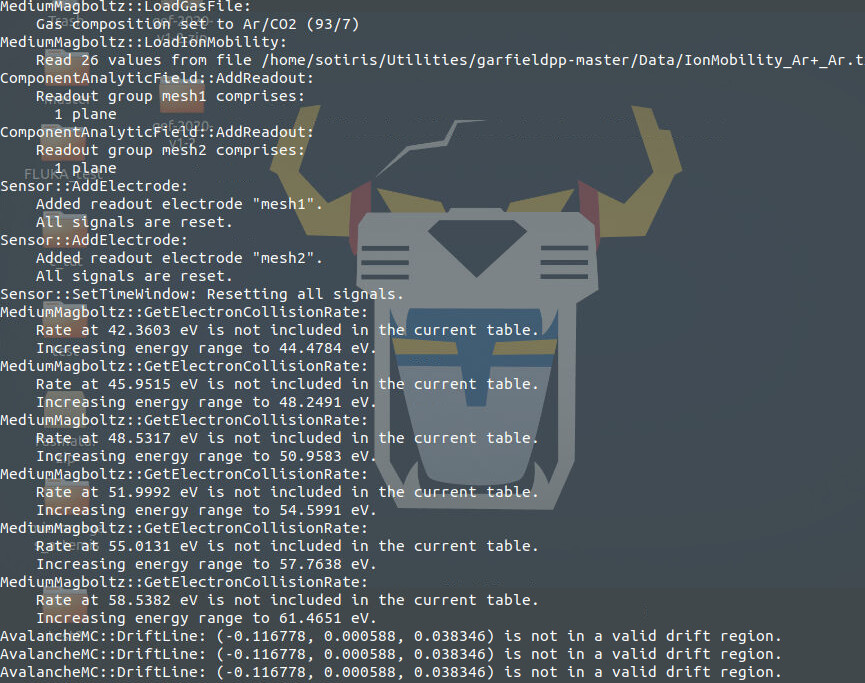
  gas.LoadGasFile("donegas.gas");
  const std::string path = std::getenv("GARFIELD_HOME");
  gas.LoadIonMobility(path + "/Data/IonMobility_Ar+_Ar.txt");

  // Build the Micromegas geometry.
  // We use separate components for drift and amplification regions. 

  ComponentAnalyticField cmpD;
  ComponentAnalyticField cmpA; 
  cmpD.SetMedium(&gas);
  cmpA.SetMedium(&gas);
  // NO magetic field [Tesla].

  // 500 um amplification gap. 

  constexpr double yMesh = 0.005;
  constexpr double vMesh = -300.;
  cmpA.AddPlaneY(yMesh, vMesh, "mesh1");
  cmpA.AddPlaneY(0., 0., "pad");

  // 6 mm drift gap.

  constexpr double yDrift = yMesh + 0.6; 
  constexpr double vDrift = -800.; 
  cmpD.AddPlaneY(yDrift, vDrift, "drift");
  cmpD.AddPlaneY(yMesh, vMesh, "mesh2");

  cmpA.AddReadout("mesh1");
  cmpD.AddReadout("mesh2");

  // Assemble a sensor.

  Sensor sensor;
  sensor.AddComponent(&cmpD); 
  sensor.AddComponent(&cmpA); 
  sensor.SetArea(-4.75, 0., -4.75, 4.75, yDrift, 4.75);
  sensor.AddElectrode(&cmpA, "mesh1"); 
  sensor.AddElectrode(&cmpD, "mesh2");

  // Set the time window [ns] for the signal calculation.
  const double tMin = 0.; 
  const double tMax = 220.; 
  const double tStep = 0.05; 
  const int nTimeBins = int((tMax - tMin) / tStep); 
  sensor.SetTimeWindow(0., tStep, nTimeBins);

  // Set the delta reponse function.
  if (!readTransferFunction(sensor)) return 0;
  sensor.ClearSignal();

  TrackSrim track;
  track.SetSensor(&sensor);
  // Read SRIM output from file.
  const std::string file = "alpha in 93ar-7co2 0.01-5mev.txt";
  if (!track.ReadFile(file)) {
    std::cerr << "Reading SRIM file failed.\n";
    return 0;
  }
  // Set the initial kinetic energy of the particle (in eV).
  track.SetKineticEnergy(5e6);					
  // Set the W value and Fano factor of the gas.
  track.SetWorkFunction(30.0);							
  track.SetFanoFactor(0.3);							
  // Set A and Z of the gas (not sure what's the correct mixing law). how to compute a and z in mixed gases	
  const double za = 0.93 * (18. / 40.) + 0.07 * (22. / 44.);
  track.SetAtomicMassNumbers(22. / za, 22);	
  track.SetTargetClusterSize(500); 

  // RKF integration.
  DriftLineRKF drift;
  drift.SetSensor(&sensor);
  //drift.SetGainFluctuationsPolya(0., 20000.);
  drift.EnableSignalCalculation();

 /*
  TCanvas* cS = nullptr;
  ViewSignal signalView;
  constexpr bool plotSignal = true;
  if (plotSignal) {
    cS = new TCanvas("cS", "", 600, 600);
    signalView.SetCanvas(cS);
    signalView.SetSensor(&sensor);
    signalView.SetLabelY("signal [fC]");
  } 
*/
  std::ofstream outfile1;
  outfile1.open("signal.txt");

  const unsigned int nTracks = 200;

  for (unsigned int j = 0; j < nTracks; ++j) {
    sensor.ClearSignal();
    track.NewTrack(0, yDrift, 0, 0, 1.023, 0.0, 0);
    double xc = 0., yc = 0., zc = 0., tc = 0., ec = 0., extra = 0.;
    int nc = 0;
    while (track.GetCluster(xc, yc, zc, tc, nc, ec, extra)) {
      drift.SetElectronSignalScalingFactor(nc);
      for (int k = 0; k < nc; ++k) {
	drift.DriftElectron(xc, yc, zc, tc);
	drift.DriftIon(xc, yc, zc, tc);
      }
    }               
    sensor.ConvoluteSignals();


    const double qmesh1 = sensor.GetSignal("mesh1", nTimeBins - 1);  
    const double qmesh2 = sensor.GetSignal("mesh2", nTimeBins - 1); 
    const double qemesh1 = sensor.GetElectronSignal("mesh1", nTimeBins - 1);
    const double qemesh2 = sensor.GetElectronSignal("mesh2", nTimeBins - 1); 
  
    outfile1 << qmesh2 << " " << qmesh1 << " " << qemesh1 << " " <<  qemesh2 << "\n";
     
   }
   outfile1.close();

   app.Run(kTRUE);
}

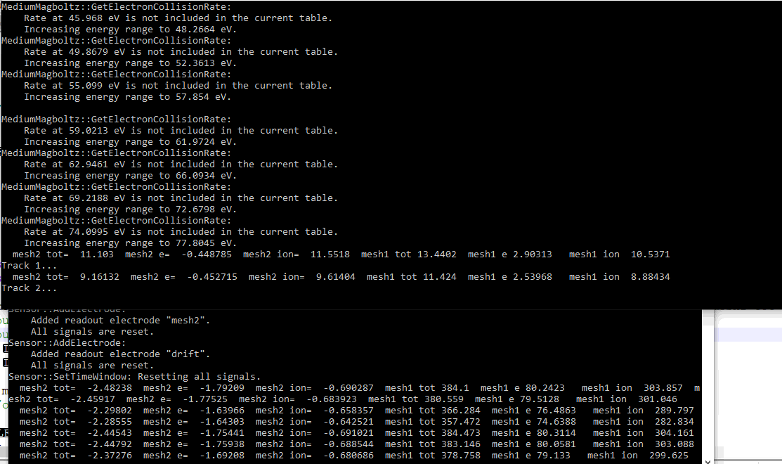
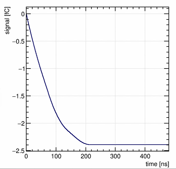
And the outputs for the signal:
signal.txt (4.1 KB)

Hi,
apologies for the long delay!
(1) I think it’s a reasonable approach in your case. The α particle will produce a large number of electron/ion pairs in the gas so it’s probably an overkill to use AvalancheMicroscopic because most of the fluctuations will be washed out.
To include the signal from the ions created in the electron avalanche in the calculation, you can add a line

drift.EnableIonTail();

(2) It’s a direction vector.
(4) For a given starting point, DriftLineRKF will always calculate the same drift line (and the same induced signal, unless you switch on gain fluctuations). So the most efficient approach would be to simulate only one electron and ion drift line per cluster and scale the signal according to the cluster size (number of electron/ion pairs in the cluster), i. e. ne:

while (track.GetCluster(xc, yc, zc, tc, nc, ec, extra)) {
  drift.SetElectronSignalScalingFactor(nc);
  drift.DriftElectron(xc, yc, zc, tc);
  drift.SetIonSignalScalingFactor(nc);
  drift.DriftIon(xc, yc, zc, tc);
}

Will reply to question (3) in a separate post…

Hello!
No problem,thank you for your response.Well:

  1. Just to make sure I get it right.There is the approach I used (with DriftLineRKF) and there is also a way to do it using AvalancheMicroscopic for the electrons( and AvalancheMC for the ions at the same time?) which is more precise but would overkill in my occation?
    I saw that AvalancheMicroscopic and AvalancheMC use microscopic and macroscopic Monte Carlo simulation respectively.Does the same happen with DriftlineRKF or by using it I lose the Monte Carlo part?
    Thank you for the ion tale information.It was useful and I had missed this in the function list.I added this one to my code.

  2. I know it maybe sounds silly but could you please be more specific about the direction vector?Which values can dx,dy and dz take?Perhaps you could give me a simple example,different than the perpendicular trajectory which exist in the examples.This one is the most important,if the answer is easy and you could,please tell me even separately of the other answers.

  3. Ok,looking forward.

  4. Changed that too.It saves me a lot of time.Thank you!

Thank you again for your answers and I am sorry for the long posts.I am just trying to understand the code.

Hi,
the strange signal you observed was due to a kind of bug in the ComponentAnalyticField class which manifested itself in your example since it has two parallel-plate geometries glued together. That part should be fixed now. I think I’ll also need to fix the “feature” that the simulation of the electron ion drift lines doesn’t stop when the electron/ion crosses the plane. Which is convenient in your case but I think it’s more of a bug than a feature.

Long story short, I’ve attached a somewhat modified version of your program that should do the trick.
It does the simulation of the electron and ion drift lines in two stages. First it simulates the drift of the primary electrons and ions in the drift gap (with the amplification gap “switched off”). Then it takes the end point of each electron drift line and simulates the avalanche (including the ion tail) in the amplification gap. The signs and relative magnitude of the induced charge now seems more reasonable. Let me know if you spot anything strange…
By the way, the program also plots the drift lines but you’ll want to switch that off (constexpr bool plotDrift = false;) when you simulate multiple tracks.

To follow up on your first question: with DriftLineRKF there is no random/Monte Carlo element in the drift line simulation. For a given starting point, all electrons/ions will go at the same end point.

  1. It’s a vector collinear with the direction in which you want the particle to fly. It doesn’t have to be normalized to 1 (the normalization is done internally). So if you want the particle to fly in the negative y-direction use e. g. (0, -1, 0). If you want it to be at an angle of 45° in the xz plane, use e. g. (1, 0, 1).

Hope that helps…
mm.C (4.3 KB)

Hello,

thank you for the programm you attached,both the results and plots are making more sense now I think.Based on the results,I have some more questions.

  1. Running the programm I am sending below (signalrkf.C), I am getting this output:
    mesh2 tot= -4.9747 mesh2 e= -2.43219 mesh2 ion= -2.54251 mesh1 tot 596.963 mesh1 e 291.862 mesh1 ion -2.54251.
    a) Now,I am finally getting electron signal and also,GetSignal=GetIonSignal+GetElectronSignal but only for mesh2.Why not in mesh1 also?The values for mesh1 seem strange.
    b) How can the ion and electron signal be both negative for mesh2 ?Maybe am I missing some physics theory here or is it about the programm?

  2. About the direction again:
    you said dx dy dz is a vector collinear with the direction in which I want the particle to fly.I tested this and the results are good.I will give an example to make sure I get it right.I wanted my particle to fly at 60 degrees from y axis,into positive x direction and so my set of parametres for the direction vector is (dx,dy,dz)=(1.732,-1,0).Does this seem reasonable to you?I double tested this for the positive z direction (dx,dy,dz)=(0,-1,1.732) and the signal is the same,as it should be.I observe the following:
    a) The same,60 degrees angle should be created when this set of parameters is being used:(dx,dy,dz)=(0.866,-0.5,0).But,when I try this,I see a difference of the order of 7% at the signal,compared to the signal I gain when (dx,dy,dz)=(1.732,-1,0).
    b) as the angle is getting bigger,the signal calculation is not always calculating.For example,for a small angle (30 degrees),I am getting results like: 4.7, 4.6, 4.3, 5.2, 5.3, 0, 4.5, 4.8 etc.
    For 60 degrees: 5.7, 5.6, 0.03, 5.3, 6.2, 0.02, 6.3, 0, 4.5, 4.8
    For very big angles (89 degrees,when (dx,dy,dz)=(57,-1,0) ) : 0, 0, 0, 0, 0, 20.2,0, 0.These are not real numbers of course,I am sending you figures of the real results,for 10 and 80 degrees (first two pictures).Can that be fixed or maybe should I add a break command in the loop so when the signal is <1 (or something) it should not be taken into account?
    c) In the same pictures,do you know what does “DriftLineRKF::DriftLine:No valid field at initial position.” mean?.I tried to to fix this using a trick I found in the programm you send me.You use y=Ymesh-1.e-10 for electrons in the amplification region (to avoid having a starting point on the plane I suppose) and I did the same for the drift region setting y=Ydrift-1.e-10 but the error still occurs.

  3. I am interested in the Monte Carlo part.Normally,I am expecting more accurate results using Monte Carlo than RKF integration,right?I am trying to make that happen (to also see the differences between the two methods).My first attempt is shown in signalmc.C where,I adjust the programm you send me,trying to replace DriftLineRKF with AvalancheMicroscopic for electrons and AvalancheMC for the ions.The programm does not work correct,giving the ouput I am sending you (last picture).That make sense,there are many faults,I have not studied it well yet,but I am sending it for telling me your opinion.It will surely take more time with avalanches method,but If the results are even more realistic,I would like to try it.

signalrkf.C (4.9 KB)
signalmc.C (5.3 KB)


  1. (a) I think that’s simply a typo in your program:
const double ionmesh1 = sensor.GetIonSignal("mesh2", nTimeBins - 1);
const double ionmesh2 = sensor.GetIonSignal("mesh2", nTimeBins - 1);

(b) That makes sense. An electron drifting towards the mesh and an ion drifting away from the mesh induce a signal with the same polarity.

  1. Yes, seems reasonable.
    (a) Could it be just statistical fluctuations?
    (b) Not sure, I would have to do some debugging. But I could imagine that this happens because due to straggling the ion track sometimes leaves the active area already during the first step (or one of the first steps). Can you give it a try with straggling switched off?
track.EnableTransverseStraggling(false);

(c) It means that the starting point provided to DriftLineRKF is not inside the active area. That shouldn’t really happen. In what scenario exactly do you get this message?

Re item 3:
There are two little issues with your code:

  • You need to make sure that the “drift gap” component is activated before you simulate the ion and electron drift lines in the drift gap:
for (int k = 0; k < nc; ++k) {
  sensor.EnableComponent(0, false);
  sensor.EnableComponent(1, true);
  // ...

By the way, in the latest version of the code the “feature” (or bug) that the drift lines were crossing over between two components. So (if you update to the HEAD version of the repository) you shouldn’t need this “trick” (enabling/disabling components) any more.

  • In the avalanche gap you need to use the method AvalancheElectron instead of DriftElectron if you want to simulate the electron avalanche. And you would have to explicitly calculate the drift lines of all ions produced in the avalanche to get the ion signal.

Let me try to explain a bit better why I think that using microscopic tracking is not a good choice in your case:

  • Microscopic tracking of electrons is typically used when fluctuations are important (for instance, when you need an accurate description of diffusion, especially in non-uniform fields, or when you care about gain fluctuations).
  • For the electrons in the drift gap, diffusion will just spread the arrival points of the electrons at the mesh. But that doesn’t matter in your case because you are looking at the signal induced on the mesh plane as a whole. So it really makes very little sense to use microscopic tracking for the electron drift lines in the drift gap.
  • In the avalanche gap, using microscopic tracking would have the advantage that it provides a more realistic description of gain fluctuations. But again, it doesn’t really matter in your case. Since you have some many primary electrons produced by the alpha particle (and, consequently, many avalanches), by the law of large numbers, the total signal will be close to the average. So using DriftLineRKF is perfectly fine.

Hello,

  1. a) Indeed,sorry for that.Changing that worked.
    b) Pefect.

  2. a) I checked this more carefully now,it works normally.
    b) This totally solved it! The plotdrift is different but signal seems to be the same.I will use it for many tracks and I will turn it on if I need to study or see one particular trajectory.
    c) It happens in many scenarios.I also get these in the code you send me,where I just changed i) the gas (the name only actually,it is also a 93 Ar 7 Co2 gas ), ii) the ionmobility path (ln53-54),because it is on a different directory and iii) the srim file (5 MeV α in 93Ar 7 Co2 0.01-5 Mev) and I get this message (image 1c).

  3. a) Yeah right,that crossed my mind too.There is not scalling factor here.Changed this such as the DriftElectron to AvalancheElectron and now it seems to be working and of course it is much slower,as expected.
    b) Thank you for explaining,your argumentation is reasonable and I agree.I just wanted to understand how the avalanche classes could replace the driftline in a code and now I think I did.It may not be needed in this situation particulary but I think I will use it somewhere.Also,using it in some trajectories,I could retrieve a more realistic for them,right?

As it concerns the update to the HEAD version of the repository.I also saw you added a new class,TrackTrim,which I would like to use but,I am not so familiar with updating Garfield and adding classes.If there an easy way or a link/topic that could help,just let me know.Otherwise,at the moment,this on/off feature(!) does not bother me.

Hi,

  1. c) maybe this happens when you have electron/hole pairs produced by the alpha track in the amplification gap. If you attach the SRIM output file you are using, I’ll take a look.

  2. b) Yes, in the sense that using AvalancheMicroscopic will provide a realistic simulation of gain fluctuations (AvalancheMC not necessarily though). But, since you have so many primary electrons, that doesn’t really matter.

To update your local version to the HEAD version of the repository, you just need to type git pull and then re-build the project.
You can find a description of the TRIM example on the website: TRIM | Garfield++

Hi,

  1. c) Ok,I am sending you the srim file below.
    In the SRIM example,in SRIM file (alpha_ArCO2_70_30.txt ) density is defined as 1.7800E-01 g/cm3 ( for 100% Argon ).In my example I use a density of 1.6532E-03 g/cm3 ( for my gas mixture).That’s a difference of 2 orders of magnitude.I think that there is a mistake in density at SRIM example,in case that matters.

alpha_in_93ar-7co2_0.01-5mev.txt (6.9 KB)

  1. b) I run the script with the avalanche classes (I send below),changing what you mentioned with the loop and using AvalancheElectron instead of DriftElectron.I am getting the same error (also sending it).Also,running for 10 tracks,I am getting a mean of 1.5 ± 0.3 fC(I attach the output file).Running the exact same trajectory with RKF class,gives me 4.5 ± 0.3 fC,which I think is a big difference.What do you think about this?

SignalAval.cpp (5.4 KB)
SignalAval output.txt (337 Bytes)

I saw the TRIM example you are attaching and that is why I want to use this class.When I update to HEAD version,running git pull,a process seemed to take place.But still,I try to use the new class TrackTrim by including it and then just building an object (TrackTrim track;) and is not working.I also tried to do it manually,taking the source file TrackTrim.cc from gitlab and adding it to my source folder,such as the TrackTrim.hh file in the include folder,but that did’t work either.Maybe I am missing something on re-building the project.What do you mean by that?

Hi,

you’re right, that doesn’t look right. Many thanks for pointing this out, I’ll put it on my to-do list to fix that.

I think I spotted two issues in the AvalancheMicroscopic-based program that you sent: (1) I think you mixed up DriftElectron and AvalancheElectron, and (2) you also need to simulate explicitly the drift lines of the ions produced in the avalanche.

I’ve attached a slightly modified version which (I think) should to the trick. It requires the HEAD version of the repository though (so we don’t need the “trick” to switch components on and off).
But as I said, given the large number of primary electron/ion pairs, I don’t think that simulating every single electron (including the avalanches) using microscopic tracking makes sense. Especially since we use a simple approximation for the electric field.
microscopic.cpp (6.3 KB)

What I meant is: after typing git pull to get the HEAD version of the source code, go to the Garfield++ build directory (usually $GARFIELD_HOME/build) and type cmake .. followed by make; make install.

Hello,

Following your instructions I updated to the HEAD version and now I can use TrackTrim and also now,unlike before,the track plot occurs,which are good news! I observe these:

  1. I am using the same code (I send it below) without using the “trick” and now, the error:
    "No valid field at initial position.
    DriftLineRKF::DriftLine:
    does not appear anymore! So,I think this code can be used to calculate the signal with DriftlineRKF method.Is that right or some changes are needed?(If I use the “trick” the error still occurs).

  2. Thank you for the microscopic script.I agree that simulating all the electrons is not needed here,but I want to compare the results I am getting from the two methods,to test if they are similar.Using the microscopic script you send me,I am taking the output I am sending you (first image.At the bottom of the image,the results of the RKF code for the same trajectory are also shown).The results seem strange to me because a) the total integrated signal in mesh2 (drift region) is much larger (4 times) than the signal I am taking using the RKF method 2) this time,the integrated signal is positive and the most of it is due to ions while with RKF code,the integrated signal was negative and the most of it was due to electrons.Do you have any idea why are these happening?

Generaly,using the script a) with Sensor::EnableComponents (before updating to HEAD version),b) with Sensor::EnableComponents (after updating to HEAD version),c) without Sensor::EnableComponents (after updating to HEAD version) and d) using the microscopic tracking script you send me,I am getting different results.I am sending you these results in an array (second image.The Monte Carlo calculations are taking more time so,for the microscopic script,one result occurs,that of the vertical track.Label “new” stands for “after updating to HEAD version”).

signalrkf.txt (5.9 KB)


image

Hi,
there was indeed a problem with the signal calculated using the microscopic method. Sorry for that, I should have done a more careful check, and thanks a lot for reporting it! I’ve just committed a fix that should solve the issue:

Can you do another git pull (+ re-build of the project)?

The merge request above also adds an option for the DriftLineRKF class to use the weighting potential (instead of the weighting field) for calculating the induced current. Can you switch on this option in your signalrkf program by adding a line

drift.UseWeightingPotential(true);

before or after drift.EnableSignalCalculation();? The reason for that is that the weighting potential approach is more suitable if one wants to ensure that the integrated charge is correct.

Otherwise your signalrkf program looks fine to me! I ran it (after updating to the HEAD version of Garfield++) and the signal in the drift gap seems correct (in the sense that if you integrate over a sufficiently long time, the integrated charge corresponds to the number of electron/ion pairs deposited in the drift gap). There is a little caveat though: the ions take a long time (hundreds of μs) to reach the top electrode. In the time window that you set (220 ns), you will therefore only see a small contribution to the total charge from the ions.

Hello,

  1. a) I think I rebuilt the project correctly.Running git pull,I receive the mesage:
    “fatal: not a git repository (or any parent up to mount point /mnt)
    Stopping at filesystem boundary (GIT_DISCOVERY_ACROSS_FILESYSTEM not set)”
    but the next steps with cmake … followed by make seem to work.I am sending you a screenshot of the process for confirmation.
    b) I will run the microscopic script again and I will inform you for the results.

  2. a) I added drift.UseWeightingPotential(true); and I get the error ‘class Garfield::DriftLineRKF’ has no member named ‘UseWeightingPotential’.Maybe the rebuild did not work?The process lasted 5-10 minutes and the building process seemed to go normal.
    b) Yes,thanks for the suggestion.I already have that in mind,when I want to retrieve the signal I am changing the TimeWindow.Speaking of this,after the rebuilds (and before) when I am running the code (the same as I had sent you in the previous comment) I get the pulse shown in the left of the second image.When I am running the same code with the “trick” I get the pulse shown in the right,which make more sense.Does that “curve” in the middle of the left pulse have some physics explanation or is that due to the code?


I’m afraid that means that you still have the previous version of the code (which is also why the compiler complains that the method DriftLineRKF::UseWeightingPotential does not exist).

In which directory did you type git pull? It has to be the directory to which you cloned the git repository (or one of its subdirectories).

Let’s discuss the signal shape once you have updated to the latest version of the code.

Hello,

I think I finally managed to rebuild the project.I added DriftLineRKF::UseWeightingPotential to my code (before or after DriftLineRKF::EnableSignalCalculation() does not seem to make a difference) and now the errors do not appear!I am now waiting results from the microscopic run to compare them to those from DriftlineRKF.

On the other hand,the signal shape is the same as the one I send you on the previous post.

Hi,
apologies for the delay in getting back to you. Great that the update and rebuild worked!
I can’t reproduce the signal shape you sent though. With the attached program I get a negative signal on “mesh2” and a positive one on “mesh1”. I’m quite puzzled that you got a bipolar signal (with an integrated charge of zero) as the weighting fields in the drift and avalanche gap are constant (in the approximation we use) and both electrons and ions induce a signal with the same polarity…
mesh1.pdf (44.2 KB)
mesh2.pdf (42.3 KB)
rkf.cpp (5.3 KB)

Hello,

  1. as I said in previous post,when I want to see the whole pulse,I am changing the Timewindow to 480 ns.The results I am taking for the two meshes,the drift and pad electrodes are these shown at picture 1. a) Using the DriftLineRKF::UseWeightingPotential (before or after the DriftLineRKF::EnableSignalCalculation(); ) makes no difference in the shape of the signal,these “fluctuations” still exist.b) In one of the plots I used ViewSignal::PlotSignal(“mesh1”,true,true,true,true,false); to also plot the electron and ion signal.It confuses me a little that both of them are positive while the total is both positive and negative.Is there an explanation to that?I am just asking out of curiosity.

  2. Using the microscopic script,in the updated version of Garfield,I am getting the output shown in the second picture.a) Do you know what this warning/error is? b) The results for the integrated signals look very strange and they are way different than the driftlineRKF results.

Hi,
hm, that’s bizarre. I’m afraid I can’t reproduce the bipolar signal shapes shown on your plots, irrespective of the time window. What signal shapes do you get when you run the attached program?

The fact that the electron and ion signals have the same polarity is normal. They have opposite charge but they also drift in the opposite directions.

Let’s sort out the strange signal shapes using the RKF method first and then look into the microscopic ones…

Don’t worry about the messages “Increasing energy range to … eV”. To avoid them, you could add a line like gas.SetMaxElectronEnergy(100.); to your program…

rkf.cpp (5.3 KB)

Hello,

the output of the script you send me,gives me the picture I am sending.It does not look like a pulse,maybe because it has sensor.IntegrateSignals(); and not sensor.ConvoluteSignals(); and transfer function.

I am sending you the script from which I am taking the pictures I sent you on the previous post.Can you send me the pulses you are getting when you run it?

rkf (1).cpp (6.8 KB)