Sampling parameters from RooFit result with asymmetric errors

Dear RooFit experts,

From the documentation of RooFitResult, the randomizePars method will sample parameters from the covariance matrix assuming Gaussian priors for all the parameters. However, in cases where the parameters have very asymmetric uncertainties, I suppose this method is not valid. What would be the recommended way to sample the parameters instead?

Regards,
Alkaid

Dear Alkaid,

Let me add in the loop @jonas , who could help out with this question.

Best,
D

Hi @AlkaidCheng,

I would suggest following the usual prescription for interpolating asymmetric pre-fit uncertainties, as done in HistFactory (see also page 16 of the HistFactory paper). In particular, to use the polynomial interpolation as implemented by “interpolation code 4” in the PiecewiesInterpolation class, which is used by HistFactory.

In other words, you sample from a unit Gaussian and then transform the value such that the mean and ± 1sigma of the Gaussian correspond to your best-fit parameter values and up and down variations, while making sure the interpolation is smooth (no jumps in first and second derivatives). Like this, the priors for your parameters will also have no discontinuity. Here a little demo for that, assuming you have a parameter with post-fit value 3.5 and asymmetric uncertainties (-0.4,+0.7):

void interp_demo()
{
   RooRealVar param{"param", "param", 3.5, 0, 10};
   RooRealVar alphaParam{"alpha_param", "", 0.0, -5.0, 5.0};

   RooGaussian alphaParamConstr{"alpha_param_constr", "", alphaParam, 0.0, 1.0};

   param.setAsymError(-0.4, 0.7);

   PiecewiseInterpolation interp{"interp",
                                 "",
                                 RooFit::RooConst(param.getVal()),
                                 RooArgList{param.getVal() + param.getErrorLo()},
                                 RooArgList{param.getVal() + param.getErrorHi()},
                                 RooArgList{alphaParam}};

   interp.Print("t");

   interp.setAllInterpCodes(4);

   auto hist = new TH1D{"hist", "sampled values", 1000, 0., 10.};

   TRandom3 rng;

   for (int i = 0; i < 10000000; ++i) {
      alphaParam.setVal(rng.Gaus());
      hist->Fill(interp.getVal());
   }

   auto c1 = new TCanvas{};
   hist->Draw();
   c1->Draw();


   c1->SaveAs("plot.png");
}

The little kink at the +1 sigma comes from the transition between polynomial interpolation and linear extrapolation.

Now, since you want to randomize with respect to the post-fit results I think you also want to consider the covariances. So I would fill the Gaussian samples in a vector and multiply them with the correlation matrix of your fit result, similar to how the implementation of RooFitResult::randomizePars() is multiplying with the covariance matrix. Then, you do the transformations as I described and that’s it. If you think this is a good prescription, we can even think of having this as an option to randomizePars().

If you don’t want to approximate with interpolations, and if computational cost permits, you can also use sample parameter points according to the full likelihood function (if available), for example with the Metropolis-Hastings algorithm. This is implemented in RooStats::MetropolisHastings, maybe it’s worth to try out this class.

Personally, since nuisance parameters are usually constrained by interpolated up-and down variations anyway, I would not mind doing the interpolation also for post-fit. But maybe for parameters-of-interest I would compare the interpolation also to more precise methods like Metropolis-Hastings before trusting it.

I hope these ideas help! Let us know how it goes and if you have more questions.

Cheers,
Jonas

HI @jonas ,

Thanks for the detailed reply. I gave the PiecewiseInterpolation method a try and extended your example to the correlated variable case according to your suggestion. Here’s some questions that I hope you could clarify:

  1. Since you have multiplied alpha vector by the correlation matrix (g @ Lt according to the notation of RooFitResult::randomizePars(), I suppose now that the result is no longer the number of standard deviation away from the mean of Gaussian. Therefore, the default value of boundary = 1.0 in PiecewiseInterpolation evaluation is no longer applicatble. I suppose it should be replaced by sqrt(covariance_matrix[i][i]).
  2. If I look more carefully into the implementation of interpolation code 4 or 6, I believe this line is wrong, as x should be t instead, i.e. mod = t * (S + t * A * (15 + t * t * (-10 + t * t * 3)))
  3. After these fixes, I tried to do the sampling of parameters, the results are making sense but not very good especially when the errors are very asymmetric. Below is a demo fit result that I have:
import ROOT

observable = ROOT.RooRealVar('myy', 'myy', 125, 105, 160)
observable.setBins(55)
c = ROOT.RooRealVar('c', 'c', 1, -10, 10)
base_pdf = ROOT.RooExponential('exp', 'exp', observable, c)
norm = ROOT.RooRealVar('N', 'N', 1, -float('inf'), float('inf'))
pdf = ROOT.RooAddPdf('exp_extended', '', ROOT.RooArgList(base_pdf), ROOT.RooArgList(norm))

observable.setRange('SB_Lo', 105, 120)
observable.setRange('SB_Hi', 130, 160)

bin_edges = np.linspace(105, 160, 55 + 1)
x = (bin_edges[:-1] + bin_edges[1:]) / 2
y = np.array([1201.58, 1179.01, 1140.39, 1128.87, 1111.56, 1124.37, 1098.3 ,
       1052.13, 1015.04, 1006.18,  971.46,  945.95,  931.43,  913.02,
        871.57,    0.  ,    0.  ,    0.  ,    0.  ,    0.  ,    0.  ,
          0.  ,    0.  ,    0.  ,    0.  ,  724.1 ,  699.51,  687.49,
        667.44,  657.39,  649.17,  634.78,  600.47,  586.51,  580.54,
        570.01,  588.22,  555.9 ,  540.72,  531.02,  546.06,  528.99,
        521.36,  495.24,  483.4 ,  448.63,  480.71,  454.2 ,  450.19,
        436.4 ,  413.69,  412.14,  420.22,  417.97,  404.38])
arrays = {
    'myy': x,
    'weight': y
}
dataset = ROOT.RooDataSet.from_numpy(arrays, ROOT.RooArgSet(observable), weight_name='weight')

fit_result = pdf.fitTo(dataset, ROOT.RooFit.Range('SB_Lo,SB_Hi'), ROOT.RooFit.PrintLevel(-1),
                       ROOT.RooFit.Hesse(True), ROOT.RooFit.Save(), ROOT.RooFit.Strategy(2),
                       ROOT.RooFit.AsymptoticError(True))

This gives (I refitted once)

{'c': {'value': -0.020686713133077784,
  'errors': (-0.009063431420349587, 0.0003276873353671196)},
 'N': {'value': 39929.87921962675,
  'errors': (-6416.289580898308, 223.7984340402964)}}

The distributions that I got after sampling 100,000 parameters are:

There’s also some extremely small (and negative) or extremely large values for N which is not quite satisfactory.

Do you have idea to improve on this? Or should we use MetropolisHastings?

Though I do think that it would be nice to have this implementation of randomizePars using piecewise interpolation.

Cheers,
Alkaid

Hello @jonas ,

Is there any news on this issue?

Thanks,
Alkaid

Hi @AlkaidCheng,

about your questions:

  1. About multiplying alphas with the correlation matrix: I’m sorry, I was not very precise there. You should not multiply with the correlation matrix directly, but first decompose it like done in the RooFitResult implementation and also explained on Wikipedia about sampling from multivariate Gaussian distributions. Then the problem that the projections are not normalized Gaussians anymore should be gone.
  2. About t instead of x: why do you think that? I made some plots to validate the formula, and with your suggested change I don’t even get a continuous interpolation-extrapolation boundary. Maybe you misunderstood the boundary parameter? It controls where to do the transition between interpolation and extrapolation. The default is 1.0, meaning the transitions are at +/- 1.0 sigma. How did you actually manage to change this boundary parameter? It’s actually hardcoded to 1.0 in the PiecewiseInterpolation. And I think it’s quite a natural choice. Maybe after fixing the previous point with the matrices you don’t need to change this anymore?
  3. The distributions that you have don’t look ideal indeed. My guess is that you introduced discontinuities by changing the interpolation implementation, which results in the multiple bumps in the pdf, in particular the tails.

By the way, your parameter uncertainties are so extremely asymmetric that I would not trust the interpolations without careful validation :smiley:

Hope it helps!
Jonas

Hi @jonas ,

Concerning 1: I did use the cholesky matrix in my implementation
Concerning 2: I still think the boundary should be adjusted. Please see my reproducer below. For the x -> t correction, after more careful inspection, I think the correction should instead be (high - nominal) -> (high - nominal) / boundary and (nominal - low) -> (nominal - low) / boundary

Please see below my reproducer

from typing import Optional, Union
import numpy as np

import ROOT

observable = ROOT.RooRealVar('myy', 'myy', 125, 105, 160)
observable.setBins(55)
c = ROOT.RooRealVar('c', 'c', 1, -10, 10)
base_pdf = ROOT.RooExponential('exp', 'exp', observable, c)
norm = ROOT.RooRealVar('N', 'N', 1, -float('inf'), float('inf'))
pdf = ROOT.RooAddPdf('exp_extended', '', ROOT.RooArgList(base_pdf), ROOT.RooArgList(norm))

observable.setRange('SB_Lo', 105, 120)
observable.setRange('SB_Hi', 130, 160)

bin_edges = np.linspace(105, 160, 55 + 1)
x = (bin_edges[:-1] + bin_edges[1:]) / 2
y = np.array([1201.58, 1179.01, 1140.39, 1128.87, 1111.56, 1124.37, 1098.3 ,
       1052.13, 1015.04, 1006.18,  971.46,  945.95,  931.43,  913.02,
        871.57,    0.  ,    0.  ,    0.  ,    0.  ,    0.  ,    0.  ,
          0.  ,    0.  ,    0.  ,    0.  ,  724.1 ,  699.51,  687.49,
        667.44,  657.39,  649.17,  634.78,  600.47,  586.51,  580.54,
        570.01,  588.22,  555.9 ,  540.72,  531.02,  546.06,  528.99,
        521.36,  495.24,  483.4 ,  448.63,  480.71,  454.2 ,  450.19,
        436.4 ,  413.69,  412.14,  420.22,  417.97,  404.38])
arrays = {
    'myy': x,
    'weight': y
}
dataset = ROOT.RooDataSet.from_numpy(arrays, ROOT.RooArgSet(observable), weight_name='weight')

fit_args = [ROOT.RooFit.Range('SB_Lo,SB_Hi'), ROOT.RooFit.PrintLevel(-1),
            ROOT.RooFit.Hesse(True), ROOT.RooFit.Save(), ROOT.RooFit.Strategy(2),
            ROOT.RooFit.AsymptoticError(True)]

fit_result = pdf.fitTo(dataset, *fit_args)

def get_covariance_matrix(fit_result):
    data = fit_result.covarianceMatrix()
    array = data.GetMatrixArray()
    nrows = data.GetNrows()
    ncols = data.GetNcols()
    cov_matrix = np.frombuffer(array, dtype='float64', count=nrows * ncols).reshape((nrows, ncols))
    return cov_matrix

# covariance matrix
C = get_covariance_matrix(fit_result)
# > print(C)
# > [[ 4.11727600e+07 -2.15903749e+01]
# >  [-2.15903749e+01  8.21503626e-05]]
# cholesky matrix
# here L is same as _Lt in https://github.com/root-project/root/blob/master/roofit/roofitcore/src/RooFitResult.cxx#L365
L = np.linalg.cholesky(C)
# > print(L)
# > [[ 6.41660034e+03  0.00000000e+00]
# >  [-3.36476853e-03  8.41597857e-03]]

# Sample Gaussian vector, shape = (n_sample, n_param)
np.random.seed(1234)
G = np.random.normal(size=(10, 2))
# > print(G)
# > [[ 4.71435164e-01 -1.19097569e+00]
# >  [ 1.43270697e+00 -3.12651896e-01]
# >  [-7.20588733e-01  8.87162940e-01]
# >  [ 8.59588414e-01 -6.36523504e-01]
# >  [ 1.56963721e-02 -2.24268495e+00]
# >  [ 1.15003572e+00  9.91946022e-01]
# >  [ 9.53324128e-01 -2.02125482e+00]
# >  [-3.34077366e-01  2.11836468e-03]
# >  [ 4.05453412e-01  2.89091941e-01]
# >  [ 1.32115819e+00 -1.54690555e+00]]

# according to https://root.cern.ch/doc/master/TVectorT_8cxx_source.html#l00990
# the line g*= (*_Lt) : https://github.com/root-project/root/blob/master/roofit/roofitcore/src/RooFitResult.cxx#L376
# will call cblas_dgemv, which does _Lt * g
# if we want to multiply multiple vectors G, it's equivalent to doing
# G * _Lt.T -> G @ L.T in our notation
R = G @ L.T
# > print(R)
# > [[ 3.02501103e+03 -1.16094961e-02]
# >  [ 9.19310803e+03 -7.45199898e-03]
# >  [-4.62372992e+03  9.89095859e-03]
# >  [ 5.51563531e+03 -8.24928422e-03]
# >  [ 1.00717347e+02 -1.89272032e-02]
# >  [ 7.37931963e+03  4.47859246e-03]
# >  [ 6.11709993e+03 -2.02185523e-02]
# >  [-2.14364094e+03  1.14192112e-03]
# >  [ 2.60163250e+03  1.06873470e-03]
# >  [ 8.47734411e+03 -1.74641155e-02]]
# note the one-sigma range of this R is definitely not (-1, 1)

parameters = [param for param in fit_result.floatParsFinal()]
# nominal value of parameters
V0 = np.array([param.getVal() for param in parameters])
# > print(V0)
# > [ 3.99293343e+04 -2.06860695e-02]

Err = np.array([[param.getErrorLo(), param.getErrorHi()] for param in parameters])
# > print(Err)
# > [[-6.41660034e+03  2.23800563e+02]
# >  [-9.06368372e-03  3.27688567e-04]]

# if I don't do any interpolation:
V_no_interp = V0 + R
# > print(V_no_interp)
# > [[ 4.29543454e+04 -3.22955657e-02]
# >  [ 4.91224424e+04 -2.81380685e-02]
# >  [ 3.53056044e+04 -1.07951109e-02]
# >  [ 4.54449697e+04 -2.89353537e-02]
# >  [ 4.00300517e+04 -3.96132727e-02]
# >  [ 4.73086540e+04 -1.62074771e-02]
# >  [ 4.60464343e+04 -4.09046218e-02]
# >  [ 3.77856934e+04 -1.95441484e-02]
# >  [ 4.25309668e+04 -1.96173348e-02]
# >  [ 4.84066784e+04 -3.81501850e-02]]
# will be roughly gaussian with the correct sigma and mean

# now do the interpolation

# implementation according to https://root.cern/doc/master/MathFuncs_8h_source.html#l00213
# with some correction:
# (high - nominal) -> (high - nominal) / boundary
# (nominal - low) -> (nominal - low) / boundary
def additive_polynomial_linear_extrapolation(
    x: Union[float, np.ndarray], nominal: float, low: float, high: float, boundary: float,
):
    x = np.asarray(x, dtype=np.float64)
    mod = np.zeros_like(x)
    mask1 = x >= boundary
    mask2 = x <= -boundary
    mask3 = ~(mask1 | mask2)

    mod[mask1] = x[mask1] * (high - nominal) / boundary
    mod[mask2] = x[mask2] * (nominal - low) / boundary
    if np.any(mask3):
        t = x[mask3] / boundary
        eps_plus = (high - nominal) / boundary
        eps_minus = (nominal - low) / boundary
        S = 0.5 * (eps_plus + eps_minus)
        A = 0.0625 * (eps_plus - eps_minus)
        mod[mask3] = x[mask3] * (S + t * A * (15 + t**2 * (-10 + t**2 * 3)))

    return mod

# case 1: set boundary to the default value of 1
R_trans_boudnary_1 = np.zeros_like(R)
for i, param in enumerate(parameters):
    nominal = param.getVal()
    low = nominal + param.getErrorLo()
    high = nominal + param.getErrorHi()
    boundary = 1.0
    R_trans_boudnary_1[:, i] = additive_polynomial_linear_extrapolation(R[:, i], nominal=nominal, low=low, high=high, boundary=boundary)

# > print(R_trans_boudnary_1)
# > [[ 6.76999171e+05 -5.56183018e-05]
# >  [ 2.05742275e+06 -3.54470407e-05]
# >  [-2.96686270e+07  4.56436535e-05]
# >  [ 1.23440229e+06 -3.92933592e-05]
# >  [ 2.25405989e+04 -9.18094810e-05]
# >  [ 1.65149588e+06  2.08657935e-05]
# >  [ 1.36901041e+06 -9.82870506e-05]
# >  [-1.37548872e+07  5.35142356e-06]
# >  [ 5.82246817e+05  5.00908818e-06]
# >  [ 1.89723438e+06 -8.45034077e-05]]
# the scaling of R_trans_boudnary_1 is obviously not correct


# case 2: set boundary to sqrt(C_ii)
R_trans_boudnary_sqrtCii = np.zeros_like(R)
for i, param in enumerate(parameters):
    nominal = param.getVal()
    low = nominal + param.getErrorLo()
    high = nominal + param.getErrorHi()
    boundary = np.sqrt(C[i, i])
    R_trans_boudnary_sqrtCii[:, i] = additive_polynomial_linear_extrapolation(R[:, i], nominal=nominal, low=low, high=high, boundary=boundary)

# > print(R_trans_boudnary_sqrtCii)
# > [[ 4.53363029e+02 -1.16094961e-02]
# >  [ 3.20640626e+02 -7.40801203e-03]
# >  [-4.52612470e+03  3.57597876e-04]
# >  [ 2.08911318e+02 -8.24255141e-03]
# >  [ 5.06849388e+01 -1.89272032e-02]
# >  [ 2.57378642e+02  6.22240610e-04]
# >  [ 2.14078889e+02 -2.02185523e-02]
# >  [-1.71057236e+03  4.62971299e-04]
# >  [ 4.91206241e+02  4.40866735e-04]
# >  [ 2.95675947e+02 -1.74641155e-02]]

V_interap_boundary_1 = V0 + R_trans_boudnary_1
# > print(V_interap_boundary_1)
# > [[ 7.16928506e+05 -2.07416878e-02]
# >  [ 2.09735208e+06 -2.07215166e-02]
# >  [-2.96286976e+07 -2.06404259e-02]
# >  [ 1.27433162e+06 -2.07253629e-02]
# >  [ 6.24699332e+04 -2.07778790e-02]
# >  [ 1.69142522e+06 -2.06652037e-02]
# >  [ 1.40893974e+06 -2.07843566e-02]
# >  [-1.37149579e+07 -2.06807181e-02]
# >  [ 6.22176152e+05 -2.06810604e-02]
# >  [ 1.93716372e+06 -2.07705729e-02]]

V_interap_boundary_sqrtCii = V0 + R_trans_boudnary_sqrtCii
# > print(V_interap_boundary_sqrtCii)
# > [[ 4.03826974e+04 -3.22955657e-02]
# >  [ 4.02499750e+04 -2.80940816e-02]
# >  [ 3.54032096e+04 -2.03284717e-02]
# >  [ 4.01382457e+04 -2.89286209e-02]
# >  [ 3.99800193e+04 -3.96132727e-02]
# >  [ 4.01867130e+04 -2.00638289e-02]
# >  [ 4.01434132e+04 -4.09046218e-02]
# >  [ 3.82187620e+04 -2.02230982e-02]
# >  [ 4.04205406e+04 -2.02452028e-02]
# >  [ 4.02250103e+04 -3.81501850e-02]]

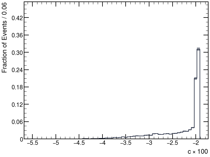
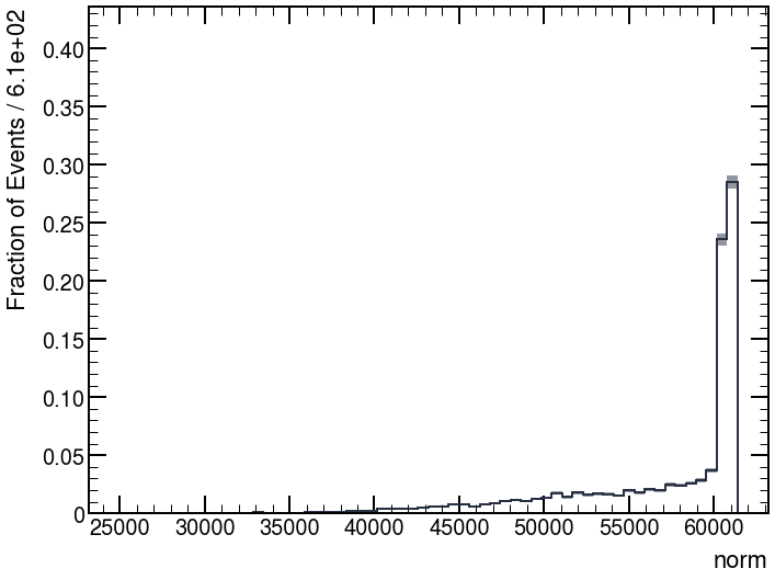
Now, the corrected distributions become:


Do you think the above implementation is correct?

Thanks,
Alkaid

Nice code, I think it’s almost correct!

But we’re still talking past each other with the correlation vs. covariance matrix.

What I’m saying is in case of doing the interpolations, your Gaussian samples after introducing the correlations with R = G @ L.T still need to be normalized as you realized. If you decompose the covariance matrix this is not the case indeed, but if you use the correlation matrix this is the case, because the correlation matrix is like a normalized covariance matrix. So you need to change this:

    data = fit_result.covarianceMatrix()

to

    data = fit_result.correlationMatrix()

If you don’t do the interpolation, using the covariance matrix is correct though, like in randomizePars().

About your suggested correction to the interpolation code with the boundary. Maybe you are right, but it depends on how the “boundary” parameter is actually defined. It’s not documented anywhere, and it’s also not used in RooFit, so we can’t infer now what it meant.

Right now, the code is such that high and low give you the variations at +/-1, independent of where you make the boundary between polynomial interpolation and linear extrapolation. You interpret it such that high and low are the variations at the boundary. In RooFit, I would suggest to leave it what it is now, because people usually bookkeep the +/-1 sigma variations.

Does that make sense maybe?

Nice code by the way! You mastered ROOT and NumPy :+1:

Thanks @jonas ,

That makes a lot of sense now. I used the covariance matrix because it’s what is used in the RooFit implementation. I believe the outcome will be the same if I used correlation matrix instead (with the advantage that you can use boundary = 1).

I will be happy to see some form of this being implemented in randomizePars, though it is not urgent.

Cheers,
Alkaid

This topic was automatically closed 14 days after the last reply. New replies are no longer allowed.