Dear all,
I am implementing a toy MC study for a model with two signals and a background:
Nexp = f1 * sgn1 + f2 * sgn2 + (1 - f1 -f2)*bkg
where the background is affected by a shape systematic through a nuisance parameter alpha.
I have constraints on both alpha and on the signal fractions: the constraint on alpha is a simple gaussian and the one on the fractions is a two dimensional gaussian with correlation (this is implemented through a RooMultiVarGausssian). To perform the toy MC experiments through RooMCStudy, and taking into account the constraints, I am following the prescriptions of this tutorial:
https://root.cern/doc/master/rf804__mcstudy__constr_8C.html
The problem I have is appearing when some of the toys are produced with “unphysical” values of the fractions (i.e. f1 + f2 > 1): here is a printout of one of these toys
  1) RooRealVar::     alpha = 5 +/- 0.00609041
  2) RooRealVar::        f1 = 1 +/- 0.000510215
  3) RooRealVar::        f2 = 0.763207 +/- 0.00668681
  4) RooRealVar::       NLL = 6975.17
  5) RooRealVar::      ngen = 2000
  6) RooRealVar:: alpha_gen = 1.53497 +/- 0.0663869
  7) RooRealVar::    f1_gen = 0.79024 +/- 0.0061129
  8) RooRealVar::    f2_gen = 0.468616 +/- 0.00518298
  9) RooRealVar::  alphaerr = 0.00609041
 10) RooRealVar:: alphapull = 568.932
 11) RooRealVar::     f1err = 0.000510215
 12) RooRealVar::    f1pull = 411.121
 13) RooRealVar::     f2err = 0.00668681
 14) RooRealVar::    f2pull = 44.0556
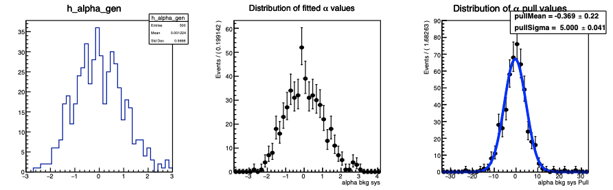
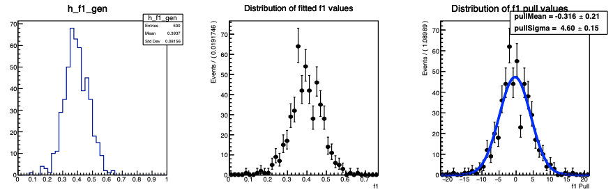
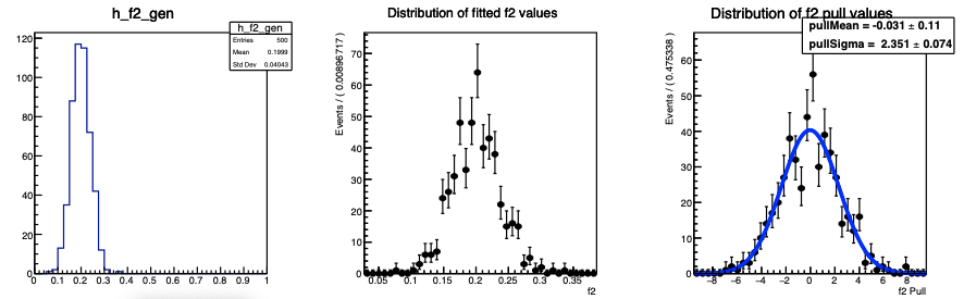
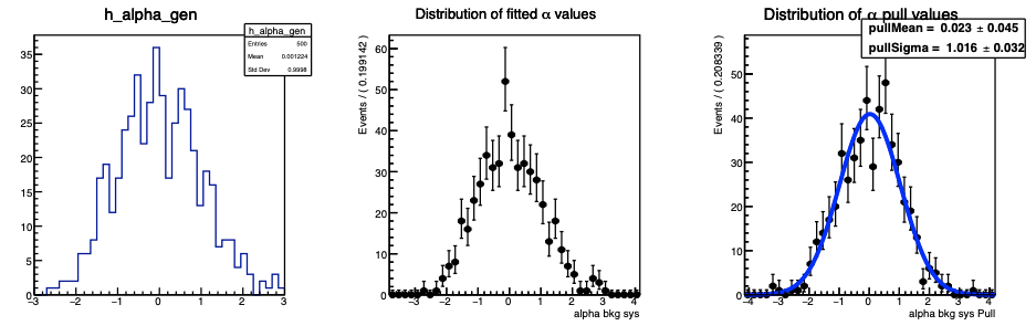
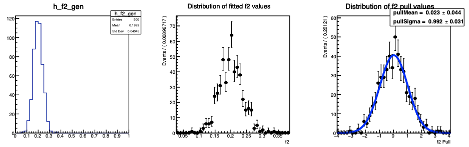
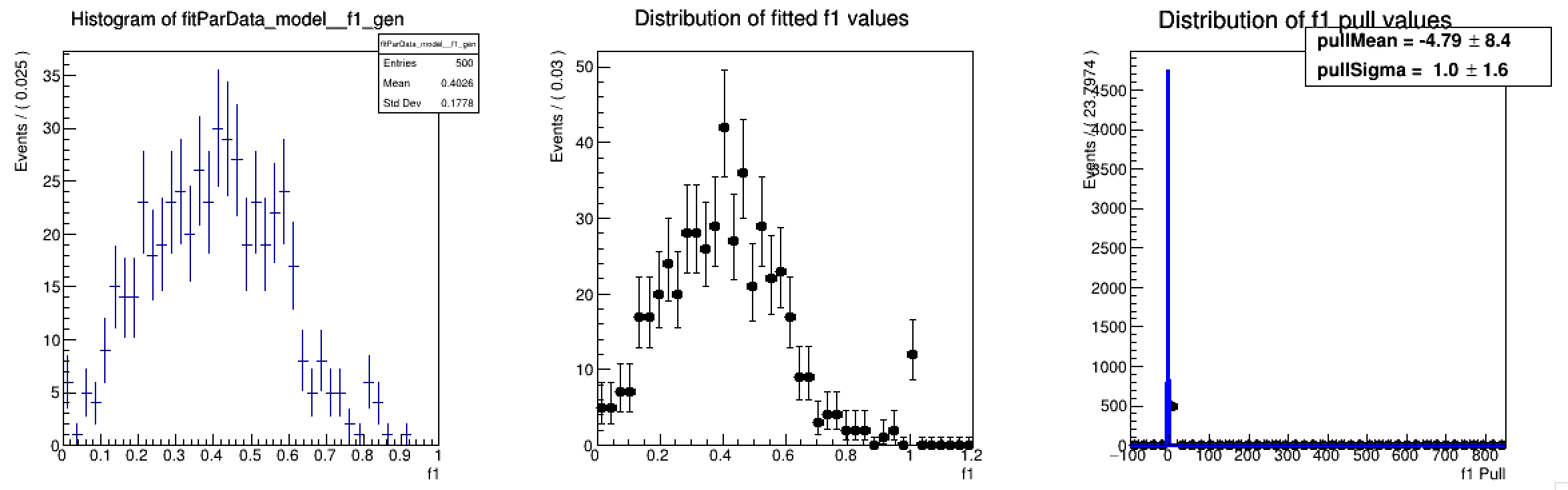
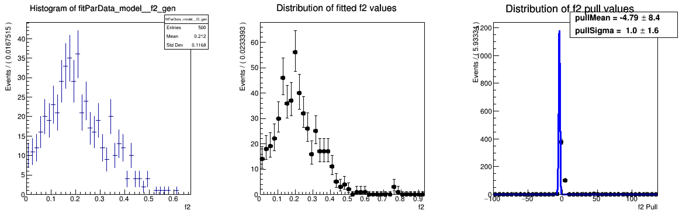
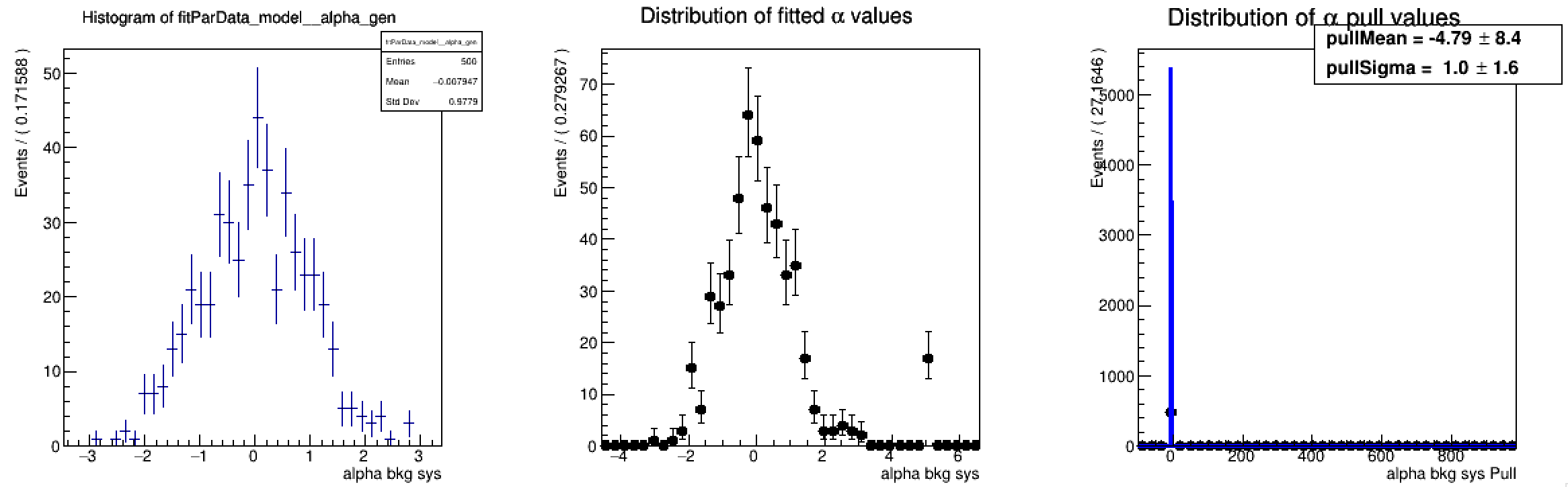
Here are the distributions I get on the parameters:
The question I have is: is there a way to configure RooMCStudy in order to reject these unphysical toys? Should I hadd some more constraints on the model?
The only solution I can think off is to write custom code deriving from RooAbsMCStudyModule to reject the unphysical values for the fractions.
Here is the code I am using:
void test_toy()
{
	// signal 1
	TH1F* hsgn1 = new TH1F("hsgn1","signal 1", 20, 0, 100);
	TF1* g = new TF1("g","[0]*exp(-(x-[1])^2/(2*[2]^2))", 0, 100);
	g -> SetParameters(100, 50, 10);
	hsgn1 -> FillRandom("g", 100000);

	// signal 2
	TH1F* hsgn2 = new TH1F("hsgn2","signal 2", 20, 0, 100);
	g -> SetParameters(100, 70, 10);
	hsgn2 -> FillRandom("g", 100000);

	// background
	TH1F* hbkg_nom = new TH1F("hbkg_nom","nominal bkg", 20, 0, 100);
	TF1* fe = new TF1("fe","[0]*exp(-[1]*x)", 0, 100);
	fe -> SetParameters(50, 0.02);
	hbkg_nom -> FillRandom("fe", 100000);

	TH1F* hbkg_p = new TH1F("hbkg_p","+1 sigma bkg", 20, 0, 100);;
	fe -> SetParameters(55, 0.03);
	hbkg_p -> FillRandom("fe", 150000);

	TH1F* hbkg_m = new TH1F("hbkg_m","-1 sigma bkg", 20, 0, 100);;
	fe -> SetParameters(45, 0.01);
	hbkg_m -> FillRandom("fe", 500000);

	// define observables
	RooRealVar e{"e", "energy", 0, 100, "MeV"};
	e.setBins(Int_t(20));

	// signal pdf
	hsgn1 -> Scale(1./hsgn1 -> Integral());
	RooDataHist dh_sgn1{"dh_sgn1", "dh_sgn1", RooArgSet{e}, hsgn1};
	RooHistPdf sgn1("sgn1", "sgn1", RooArgSet{e}, dh_sgn1);

	hsgn2 -> Scale(1./hsgn2 -> Integral());
	RooDataHist dh_sgn2{"dh_sgn2", "dh_sgn2", RooArgSet{e}, hsgn2};
	RooHistPdf sgn2("sgn2", "sgn2", RooArgSet{e}, dh_sgn2);

	// background pdf
	//
	// nominal value
	hbkg_nom -> Scale(1./hbkg_nom -> Integral());
	RooDataHist dh_bkg_nom{"dh_bkg_nom", "dh_bkg_nom", RooArgSet{e}, hbkg_nom};
	RooHistPdf bkg_0("bkg_0", "bkg_0", RooArgSet{e}, dh_bkg_nom);
	//
	// bkg +1 sigma
	hbkg_p -> Scale(1./hbkg_p -> Integral());
	RooDataHist dh_bkg_p{"dh_bkg_p", "dh_bkg_p", RooArgSet{e}, hbkg_p};
	RooHistPdf bkg_p("bkg_p", "bkg_p", RooArgSet{e}, dh_bkg_p);
	//RooHistFunc bkg_p("bkg_p", "bkg_p", RooArgSet{e}, dh_bkg_p);
	//
	// bkg -1 sigma
	hbkg_m -> Scale(1./hbkg_m -> Integral());
	RooDataHist dh_bkg_m{"dh_bkg_m", "dh_bkg_m", RooArgSet{e}, hbkg_m};
	RooHistPdf bkg_m("bkg_m", "bkg_m", RooArgSet{e}, dh_bkg_m);
	//
	// build interpolation between -1 -> +1 sigma
	RooRealVar alpha{"alpha", "alpha bkg sys", 0, -5, 5};
	PiecewiseInterpolation bkg_sys("bkg_sys", "bkg_sys", bkg_0, bkg_m, bkg_p, alpha);

	// build model
	double f1_val = 0.4;
	double f2_val = 0.2;
	RooRealVar f1{"f1", "f1", f1_val, 0, 1};
	RooRealVar f2{"f2", "f2", f2_val, 0, 1};

	RooRealSumPdf sb{"sb", "sb", RooArgSet(sgn1, sgn2, bkg_sys), RooArgList(f1, f2)};

	// introduce alpha constraint
	RooGaussian gaus_alpha("gaus_alpha", "gaus_alpha", alpha, RooFit::RooConst(0), RooFit::RooConst(1));

	// introduce f1, f2 constraint

	TMatrixDSym Vf(2);
	double sigma_f = 0.04;
	Vf(0,0) = sigma_f;
	Vf(1,1) = sigma_f/2.;
	Vf(0,1) = -0.02*sigma_f*sigma_f/2.;

	RooMultiVarGaussian mgaus_f("c_Vf", "c_Vf", RooArgList(f1, f2), RooArgList(RooFit::RooConst(f1_val), RooFit::RooConst(f2_val)), Vf);

	RooProdPdf model{"model", "model", RooArgList(sb, gaus_alpha, mgaus_f)};

	// Example of single experiment
	//
	alpha.setVal(2);
	RooDataHist* data = model.generateBinned(RooArgSet{e}, 15000, RooFit::Verbose(1));

	TCanvas* c = new TCanvas();
	c->cd();

	auto frame = e.frame(RooFit::Title("Before fit"));

	data->plotOn(frame);

	model.plotOn(frame, RooFit::LineColor(6));
	model.plotOn(frame, RooFit::LineColor(2), RooFit::Components("sgn1"));
	model.plotOn(frame, RooFit::LineColor(44), RooFit::Components("sgn2"));
	model.plotOn(frame, RooFit::LineColor(4), RooFit::Components("bkg_sys"));

	frame -> Draw();

	// fit
	f1.setVal(f1_val+0.05);
	f2.setVal(f2_val+0.05);
	alpha.setVal(0.0);
	//alpha.setConstant(kTRUE);

	auto fitres = model.fitTo(*data, RooFit::Constrain(RooArgSet(alpha, f1, f2)), RooFit::Save());

	fitres->Print();

	TCanvas* c1 = new TCanvas();
	c1->cd();

	auto frame1 = e.frame(RooFit::Title("After fit"));

	data->plotOn(frame1);

	model.plotOn(frame1, RooFit::LineColor(6));
	model.plotOn(frame1, RooFit::LineColor(2), RooFit::Components("sgn1"));
	model.plotOn(frame1, RooFit::LineColor(44), RooFit::Components("sgn2"));
	model.plotOn(frame1, RooFit::LineColor(4), RooFit::Components("bkg_sys"));

	frame1 -> Draw();

	// Toy MC (from tutorial https://root.cern/doc/master/rf804__mcstudy__constr_8C.html)
	//
	// Perform toy study with internal constraint on alpha, f1 and f2
	f1.setVal(f1_val);
	f2.setVal(f2_val);

	RooMCStudy mcs(model, e, RooFit::Constrain(RooArgSet(alpha, f1, f2)), RooFit::Silence(), RooFit::Binned(), RooFit::FitOptions(RooFit::PrintLevel(-1)));

	// Run 500 toys of 2000 events.
	// Before each toy is generated, a value for alpha, f1 and f2 is sampled from the constraint pdfs and
	// that value is used for the generation of that toy.
	mcs.generateAndFit(500, 2000);

	// Make plot of distribution of generated value of alpha parameter
	TH1 *h_alpha_gen = mcs.fitParDataSet().createHistogram("alpha_gen", -40);

	// Make plot of distribution of fitted value of alpha parameter
	RooPlot *frame2 = mcs.plotParam(alpha, RooFit::Bins(40));
	frame2 -> SetTitle("Distribution of fitted #alpha values");

	// Make plot of pull distribution on alpha
	RooPlot *frame3 = mcs.plotPull(alpha, RooFit::Bins(40), RooFit::FitGauss());
	frame3 -> SetTitle("Distribution of #alpha pull values");

	TCanvas *c2 = new TCanvas("mcstudy_alpha_constr", "mcstudy_alpha_constr", 1200, 400);
	c2 -> Divide(3);

	c2 -> cd(1);
	gPad -> SetLeftMargin(0.15);
	h_alpha_gen -> GetYaxis() -> SetTitleOffset(1.4);
	h_alpha_gen -> Draw();

	c2 -> cd(2);
	gPad -> SetLeftMargin(0.15);
	frame2 -> GetYaxis() -> SetTitleOffset(1.4);
	frame2 -> Draw();

	c2 -> cd(3);
	gPad -> SetLeftMargin(0.15);
	frame3 -> GetYaxis() -> SetTitleOffset(1.4);
	frame3 -> Draw();

	// Make plot of distribution of generated value of f1 parameter
	TH1 *h_f1_gen = mcs.fitParDataSet().createHistogram("f1_gen", -40);


	double f1pull(0), f2pull(0);
	for(auto t=0; t<500; t++)
	{
		cout << "\nN TOY = " << t << "\n" << endl;

		f1pull = mcs.fitParDataSet().get(t)->getRealValue("f1pull");
		f2pull = mcs.fitParDataSet().get(t)->getRealValue("f2pull");

		if( f1pull > 50 || f2pull > 50 )
			cout << "\nPROBLEM\n" << endl;

		mcs.fitParDataSet().get(t)->Print("V");
	}

	// Make plot of distribution of fitted value of f1 parameter
	RooPlot *frame4 = mcs.plotParam(f1, RooFit::Bins(40));
	frame4 -> SetTitle("Distribution of fitted f1 values");

	// Make plot of pull distribution on f1
	RooPlot *frame5 = mcs.plotPull(f1, RooFit::Bins(40), RooFit::FitGauss());
	frame5 -> SetTitle("Distribution of f1 pull values");

	TCanvas *c3 = new TCanvas("mcstudy_f1_constr", "mcstudy_f1_constr", 1200, 400);
	c3 -> Divide(3);

	c3 -> cd(1);
	gPad -> SetLeftMargin(0.15);
	h_f1_gen -> GetYaxis() -> SetTitleOffset(1.4);
	h_f1_gen -> Draw();

	c3 -> cd(2);
	gPad -> SetLeftMargin(0.15);
	frame4 -> GetYaxis() -> SetTitleOffset(1.4);
	frame4 -> Draw();

	c3 -> cd(3);
	gPad -> SetLeftMargin(0.15);
	frame5 -> GetYaxis() -> SetTitleOffset(1.4);
	frame5 -> Draw();

	// Make plot of distribution of generated value of f2 parameter
	TH1 *h_f2_gen = mcs.fitParDataSet().createHistogram("f2_gen", -40);

	// Make plot of distribution of fitted value of f2 parameter
	RooPlot *frame6 = mcs.plotParam(f2, RooFit::Bins(40));
	frame6 -> SetTitle("Distribution of fitted f2 values");

	// Make plot of pull distribution on f2
	RooPlot *frame7 = mcs.plotPull(f2, RooFit::Bins(40), RooFit::FitGauss());
	frame7 -> SetTitle("Distribution of f2 pull values");

	TCanvas *c4 = new TCanvas("mcstudy_f2_constr", "mcstudy_f2_constr", 1200, 400);
	c4 -> Divide(3);

	c4 -> cd(1);
	gPad -> SetLeftMargin(0.15);
	h_f2_gen -> GetYaxis() -> SetTitleOffset(1.4);
	h_f2_gen -> Draw();

	c4 -> cd(2);
	gPad -> SetLeftMargin(0.15);
	frame6 -> GetYaxis() -> SetTitleOffset(1.4);
	frame6 -> Draw();

	c4 -> cd(3);
	gPad -> SetLeftMargin(0.15);
	frame7 -> GetYaxis() -> SetTitleOffset(1.4);
	frame7 -> Draw();

}
Thanks for your help.
 )
)