Hi @jonas ,
Thanks a lot for the reply! I’m trying to use xm and dm as fundamental variables because my signal peaks in these two variables. The model pdf in the test script is used to describe a background which peaks in xm+dm only. I guess model, as a product of tPdf and xPdf, is still a valid pdf for xm and dm? It seems working in this test script:
#!/usr/bin/env python3
from ROOT import gROOT, TFile, TCanvas, RooAbsReal, RooArgSet, RooWorkspace, RooFit
def test():
w = RooWorkspace('w')
w.factory('xm[670,650,720]')
w.factory('dm[900,875,995]')
w.factory('expr::bm("xm+dm",xm,dm)')
# w.factory('Gaussian::tPdf(bm,mean[1620,1615,1625],sigma[5,0.1,25])')
# w.factory('CrystalBall::tPdf(bm,mean[1620,1615,1625],sigma[5.,0.1,10],sigma,aL[3.06,0.1,9],nL[2.43,0.1,9],aR[4.37,0.1,12],nR[8.08,0.1,12])')
w.factory('Hypatia2::tPdf(bm,l[-4.,-9,-0.6],zeta[0,0,10],fb[0],sigma[15.,0.1,20],mean[1620,1615,1625],aL[100,0.1,200],nL[2.43,0.1,10],aR[100,0.1,200],nR[8.0,0.1,10])')
w.factory('Chebychev::xPdf(xm, {a1p[0.9,0,1],a2p[0.1,0,0.5]})')
w.factory('PROD::model(tPdf, xPdf)')
w['zeta'].setConstant(True)
w['aL'].setConstant(True)
w['nL'].setConstant(True)
w['aR'].setConstant(True)
w['nR'].setConstant(True)
xm = w['xm']
dm = w['dm']
bm = w['bm']
tPdf = w.pdf('tPdf')
model = w.pdf('model')
obs = RooArgSet(xm,dm)
data = model.generate(obs, 50000)
bmv = data.addColumn(bm)
# tPdf.fitTo(data)
# bframe = bmv.frame(RooFit.Bins(100), RooFit.Range(1560,1680))
# data.plotOn(bframe)
#
# # tPdf.plotOn(bframe)
# tPdf.plotOn(bframe, RooFit.ProjWData(data))
# # tPdf.plotOn(bframe,RooFit.Normalization(data.sumEntries(), RooAbsReal.NumEvent))
# # tPdf.plotOn(bframe,RooFit.Normalization(1.0, RooAbsReal.RelativeExpected))
# # tPdf.plotOn(bframe, RooFit.Normalization(1., RooAbsReal.Relative))
# bframe.Draw()
w['a1p'].setVal(0.5)
w['a2p'].setVal(0.2)
w['mean'].setVal(1624)
w['sigma'].setVal(9)
w['l'].setVal(-1.5)
rf = model.fitTo(data,Save=True)
rf.Print("v")
c1 = TCanvas()
c1.Divide(3)
c1.cd(1)
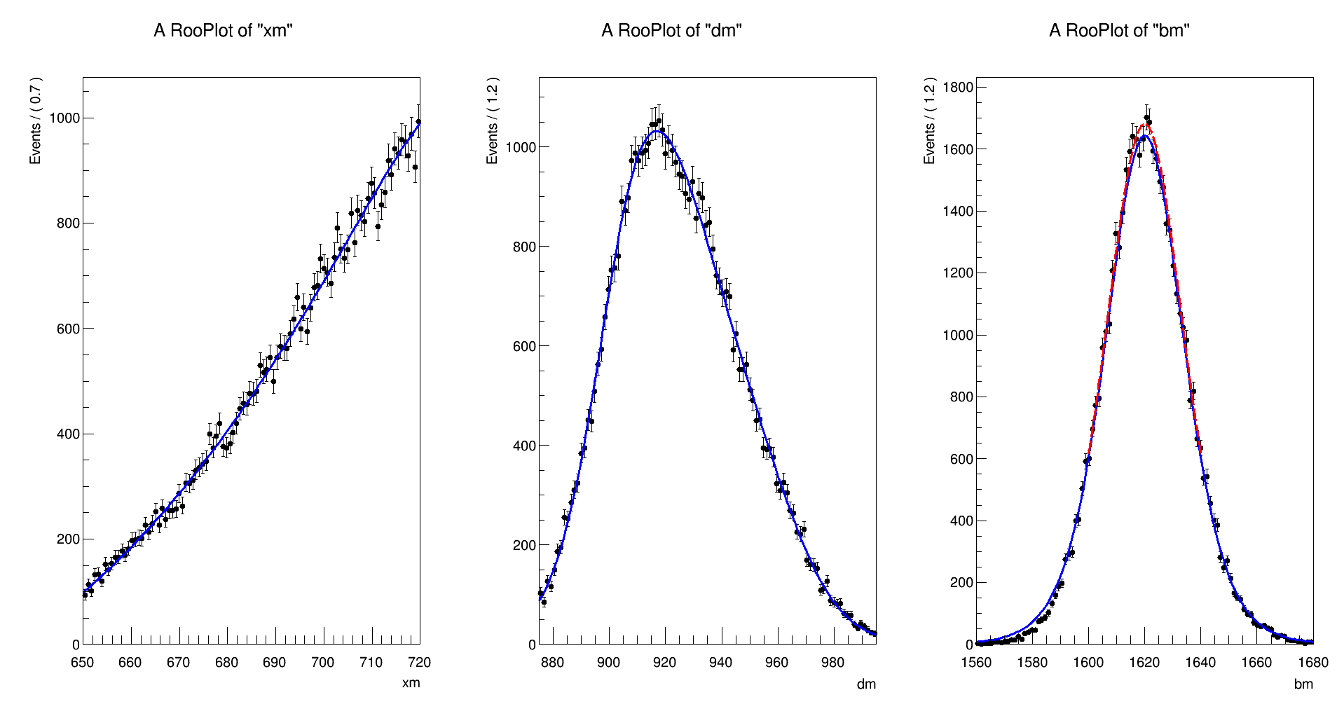
xm = w.var('xm')
xframe = xm.frame()
data.plotOn(xframe)
model.plotOn(xframe)
xframe.Draw()
c1.cd(2)
dm = w.var('dm')
dframe = dm.frame()
data.plotOn(dframe)
model.plotOn(dframe)
dframe.Draw()
c1.cd(3)
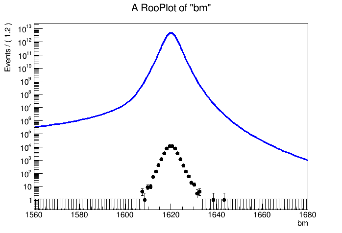
bframe = bmv.frame(Bins=100,Range=(1560,1680))
data.plotOn(bframe)
model.plotOn(bframe, RooFit.Normalization(2.e-19, RooAbsReal.Relative))
bframe.Draw()
c1.Update()
a = input('wait...')
if __name__ == '__main__':
test()
The distribution I can get is
The normalization for
xm and
dm are the default but for
bm I have to scale it by 2.e-19 to get it close to data.
Also thanks for the tips and the work behind them. They helps a lot to make my codes clear.