RooFit: Poisson constraint for nuisance parameters

Hi, I have a problem with constraints and would be very grateful for comments and corrections:

Situation:
I perform an extended, unbinned likelihood fit over ~5000 evts with 2 observables and a SUM-PDF of 20 components + 1 signal. There’s overlap between some backgrounds and the signal, so I am using constraints. The last step is a hypothesis test with the RooStats HypoTestInverter class to get an upper 90% C.L. limit on my signal.

Problem:
For all of my nuisance parameters I can calculate (by fitting sidebands and extrapolating) how many evts I expect in the data. This number can be as small as 1e-6 up to tens of evts. As the underlying data is the result of Poisson processes, I thought of using a Poisson PDF for the constraint.

Questions:
[ol]
[li] is a Poisson PDF the right one to use? Or should I use Gaussian constraints[/li]
[li] should the PDF be the discrete RooFit RooPoisson PDF or a continuous one (with an implementation of TMath::Poisson(x,µ) )?[/li]
[li] is the implementation of the global observable correct? In RooStats tutorials it is always
Gaussian(globalobs,nuisance,width) but for a Poisson PDF I believe it should be Poisson(nuisance,globalobs)[/li][/ol]

I created a minimal working example in python with a very simple model showing the basic situation (only 1d, 2 backgrounds, toy data, …):
already with this, problems occur. Fit results are completely different, depending on which constraint PDF is used (uncommented). For the discrete constraint, the fit doesn’t converge properly. And for both constraint possibilities I couldn’t perform the hypothesis test, using the ROOT StandardHypoTestInvDemo.C macro.

mwe_constraint.py (2.27 KB)

#!/usr/bin/env python
import ROOT
from ROOT import RooFit as RF
from ROOT import RooStats as RS

# Initial number of events
n_bkg1_init = 50
n_bkg2_init = 0.2
n_sig_init = 0

# Create workspace and one observable
w = ROOT.RooWorkspace("w")
x = w.factory("x[0,10]")

# Construct PDFs for signal and 2 backgrounds
sig = w.factory("Gaussian::sig(x,sig_mean[5],sig_sigma[0.5])")
bkg1 = w.factory("Polynomial::bkg1(x)")
bkg2 = w.factory("Gaussian::bkg2(x,bkg2_mean[7],bkg2_sigma[0.5])")
model = w.factory("SUM::model(n_sig[0,10]*sig,n_bkg1[0,100]*bkg1,n_bkg2[0,5]*bkg2)")

# Create constraint PDF
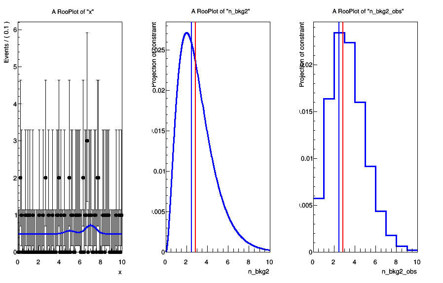
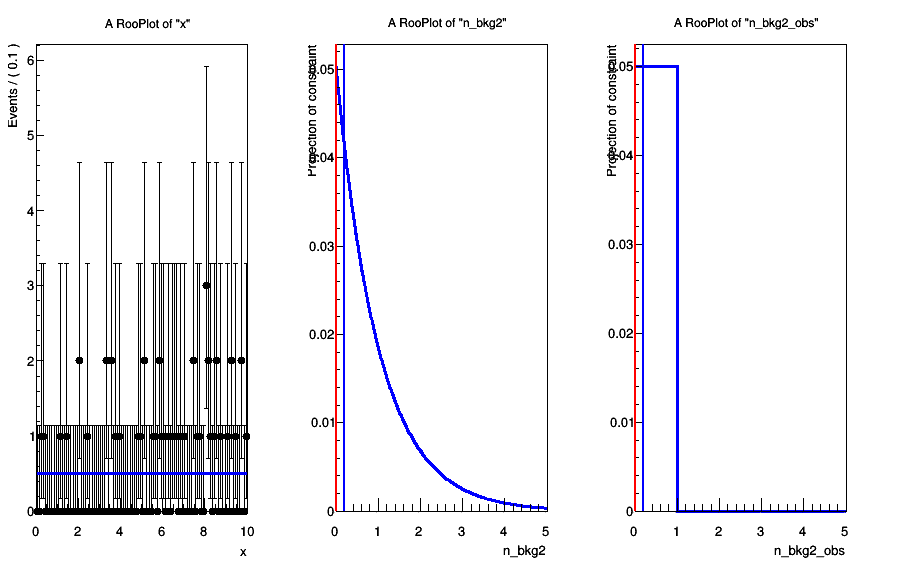
#constraint = w.factory("EXPR::constraint('TMath::Poisson(n_bkg2,n_bkg2_obs)',n_bkg2,n_bkg2_obs[0,10])")  #  continuous Poisson PDF
constraint = w.factory("Poisson::constraint(n_bkg2,n_bkg2_obs[0,5])")  # discrete Poisson PDF
cmodel = w.factory("PROD::cmodel(model,constraint)")

# Initialize number of events
w.var("n_sig").setVal(n_sig_init)
w.var("n_bkg1").setVal(n_bkg1_init)
w.var("n_bkg2").setVal(n_bkg2_init)
w.var("n_bkg2_obs").setVal(n_bkg2_init)
w.var("n_bkg2_obs").setConstant()

# Generate toy event set and fit it
data = cmodel.generate(ROOT.RooArgSet(x), RF.Name("data"))
r = cmodel.fitTo(data, RF.Minimizer("Minuit2","Migrad"), RF.Strategy(2), RF.Extended(1), RF.Constrained(), RF.Save(1))
r.Print("v")
getattr(w,"import")(data)

# Plot toy data with best fit PDF plus constraint PDF
c = ROOT.TCanvas()
c.Divide(2)
c.cd(1)
xframe = x.frame()
data.plotOn(xframe)
model.plotOn(xframe)
xframe.Draw()
c.cd(2)
bframe = w.var("n_bkg2").frame()
w.pdf("constraint").plotOn(bframe, RF.Precision(1e-5))
bframe.Draw()

# Draw line indicating the best fit for n_bkg2
c.Update()
line = ROOT.TLine()
line.SetLineColor(ROOT.kRed)
line.DrawLine(r.floatParsFinal().find('n_bkg2').getVal(), ROOT.gPad.GetUymin(), r.floatParsFinal().find('n_bkg2').getVal(), ROOT.gPad.GetUymax())


# Create RooStats model config and store it in workspace
mc = RS.ModelConfig("mc", w)
mc.SetPdf( cmodel )
mc.SetParametersOfInterest( ROOT.RooArgSet(w.var("n_sig")) )
mc.SetObservables( ROOT.RooArgSet(w.var("x")) )
mc.SetConstraintParameters( ROOT.RooArgSet(w.var("n_bkg2")) )
mc.SetNuisanceParameters( ROOT.RooArgSet(w.var("n_bkg1"),w.var("n_bkg2")) )
mc.SetGlobalObservables( ROOT.RooArgSet(w.var("n_bkg2_obs")) )
getattr(w,"import")(mc)

w.Print('v')

Hi,

If the origin of your side-band parameter is due to a number counting (Poissonian) process it is correct to add a Poisson/Gamma term for your constraint. It is a Poisson or a Gamma depending on how you interpret it.
If you have a discrete observation n (which in RooStats will be your global or normal observable) for some expected value µ, you will add a Poisson(n,µ) in your likelihood.
You interpret your nuisance also as Gamma distributed (in this case you don;t have problem with integers) and the global observable will be the alpha (or gamma as called in RooFit) and the nuisance parameter µ:
Gamma( µ, alpha, beta=1).

In your example you are inverting the Poisson parameters, it should be : Poisson(n_bkg2_obs, n_bkg2) or
Gamma(n_bkg2, n_bkg2_obs+1, 1)

Best Regards

Lorenzo

Hi Lorenzo,

thanks for your quick reply. In this case I could use Poisson constraints I guess.

At least for some of my 20 components it is. For example I have one PDF component for which I know the events to be Gaussian distributed, with half of them below my ROI. So I fit them in the sideband and expect the same number in the ROI.

I have difficulties understanding why it is defined this way around. Shouldn’t a constraint term be a distribution of that parameter? And isn’t the global observable just the expected value (thus constant)?:
I.e. L_constraint = L (theta) * Poisson(theta, µ=15) if we expect 15 evts?

How can I visualize the effect of the constraint PDF in my code example?
I changed to code slightly to plot the constraint PDF for both cases (see plot below). In one case I get a discrete distribution, in the other a continuous one. Which one is used during minimization?
(blue lines indicate the expected value (n_bkg2_init), red lines the best fit value for n_bkg2)

EDIT: With a higher input value n_bkg2_init = 2.5 the plot becomes clearer (see 1st plot below):
The distribution on the left is clearly not a Poisson distribution.

Changed code:

[code]#!/usr/bin/env python
import ROOT
from ROOT import RooFit as RF
from ROOT import RooStats as RS

Initial number of events

n_bkg1_init = 50
n_bkg2_init = 0.2
n_sig_init = 0

Create workspace and one observable

w = ROOT.RooWorkspace(“w”)
x = w.factory(“x[0,10]”)

Construct PDFs for signal and 2 backgrounds

sig = w.factory(“Gaussian::sig(x,sig_mean[5],sig_sigma[0.5])”)
bkg1 = w.factory(“Polynomial::bkg1(x)”)
bkg2 = w.factory(“Gaussian::bkg2(x,bkg2_mean[7],bkg2_sigma[0.5])”)
model = w.factory(“SUM::model(n_sig[0,10]*sig,n_bkg1[0,100]*bkg1,n_bkg2[0,10]*bkg2)”)

Create constraint PDF

constraint = w.factory(“Poisson::constraint(n_bkg2_obs[0,10],n_bkg2)”) # discrete Poisson PDF
cmodel = w.factory(“PROD::cmodel(model,constraint)”)

Initialize number of events

w.var(“n_sig”).setVal(n_sig_init)
w.var(“n_bkg1”).setVal(n_bkg1_init)
w.var(“n_bkg2”).setVal(n_bkg2_init)
w.var(“n_bkg2_obs”).setVal(n_bkg2_init)
w.var(“n_bkg2_obs”).setConstant()

Generate toy event set and fit it

data = cmodel.generate(ROOT.RooArgSet(x), RF.Name(“data”))
r = cmodel.fitTo(data, RF.Minimizer(“Minuit2”,“Migrad”), RF.Strategy(2), RF.Extended(1), RF.Constrained(), RF.Save(1))
r.Print(“v”)
getattr(w,“import”)(data)

Plot toy data with best fit PDF plus constraint PDF

line = ROOT.TLine()
line.SetLineWidth(2)

c = ROOT.TCanvas()
c.Divide(3)
c.cd(1)
xframe = x.frame()
data.plotOn(xframe)
model.plotOn(xframe)
xframe.Draw()

c.cd(2)
bframe1 = w.var(“n_bkg2”).frame()
w.pdf(“constraint”).plotOn(bframe1, RF.Precision(1e-5))
bframe1.Draw()

Draw line indicating the best fit for n_bkg2

c.Update()
line.SetLineColor(ROOT.kRed)
line.DrawLine(r.floatParsFinal().find(‘n_bkg2’).getVal(), ROOT.gPad.GetUymin(), r.floatParsFinal().find(‘n_bkg2’).getVal(), ROOT.gPad.GetUymax())
line.SetLineColor(ROOT.kBlue)
line.DrawLine(n_bkg2_init, ROOT.gPad.GetUymin(), n_bkg2_init, ROOT.gPad.GetUymax())

c.cd(3)
bframe2 = w.var(“n_bkg2_obs”).frame()
w.pdf(“constraint”).plotOn(bframe2, RF.Precision(1e-5))
bframe2.Draw()

Draw line indicating the best fit for n_bkg2

c.Update()
line.SetLineColor(ROOT.kRed)
line.DrawLine(r.floatParsFinal().find(‘n_bkg2’).getVal(), ROOT.gPad.GetUymin(), r.floatParsFinal().find(‘n_bkg2’).getVal(), ROOT.gPad.GetUymax())
line.SetLineColor(ROOT.kBlue)
line.DrawLine(n_bkg2_init, ROOT.gPad.GetUymin(), n_bkg2_init, ROOT.gPad.GetUymax())

Create RooStats model config and store it in workspace

mc = RS.ModelConfig(“mc”, w)
mc.SetPdf( cmodel )
mc.SetParametersOfInterest( ROOT.RooArgSet(w.var(“n_sig”)) )
mc.SetObservables( ROOT.RooArgSet(w.var(“x”)) )
mc.SetConstraintParameters( ROOT.RooArgSet(w.var(“n_bkg2”)) )
mc.SetNuisanceParameters( ROOT.RooArgSet(w.var(“n_bkg1”),w.var(“n_bkg2”)) )
mc.SetGlobalObservables( ROOT.RooArgSet(w.var(“n_bkg2_obs”)) )
getattr(w,“import”)(mc)

w.Print(‘v’)[/code]


If you want to interpret the constraint in this way you should use a Gamma, which is the correct distribution for the Poisson parameter.

If you interpret as an auxiliary measurement, i.e. an extra measurement and not a s constraint (i.e. a distribution in the parameter), then it should be a Poisson.

Lorenzo

Thank you again Lorenzo, I hope I now finally understand how the constraint term is working:

It is the probability of a Poisson distribution with the mean of the nuisance parameter, evaluated at the additional measurement.
So for example how probable is the measured sideband value of 10 events, if we fit 12 evts in our data (and assume that is the mean of the fitted component).