RooFit: Background component not staying constant despite RooConstVar / setConstant(true)?

[fROOTtinator]

Dear experts,

I’m working on a 2D model fit using RooFit. My model includes a signal and two background components (signal, background1, background2) and i want to include a third background component (background3) as a constant contribution.

To test this I generate a dataset from a model without the third background (model_woBG3), afterwards I create a model including the third background (model) and fit it to the dataset.
The intention is, that the third background component stays constant during the fit and the other components are adjusted.
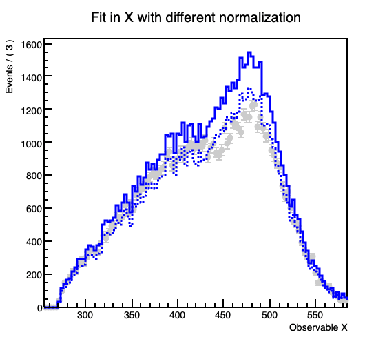
However, when I plot the fitted model and its components (background3) seems to differ slightly from the histogram I get it from, despite declaring nbkg3 as a RooConstVar.
This gets more prominent with increasing the contribution of the the background.

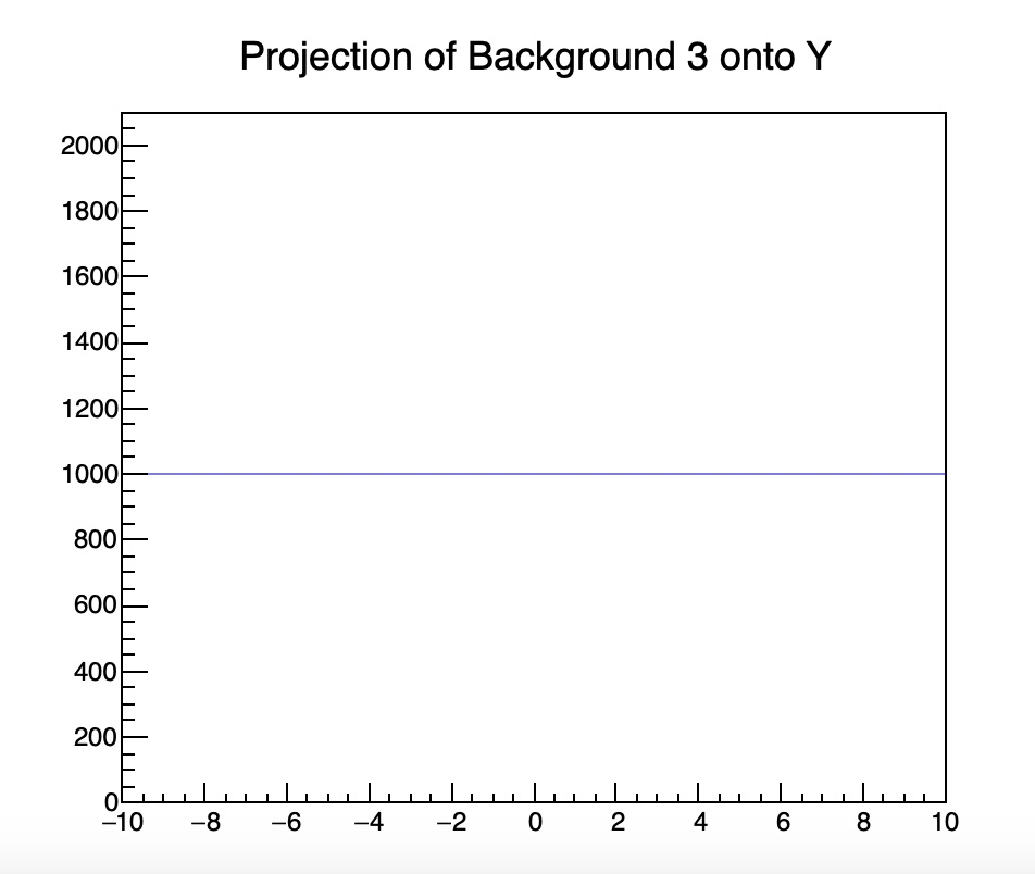
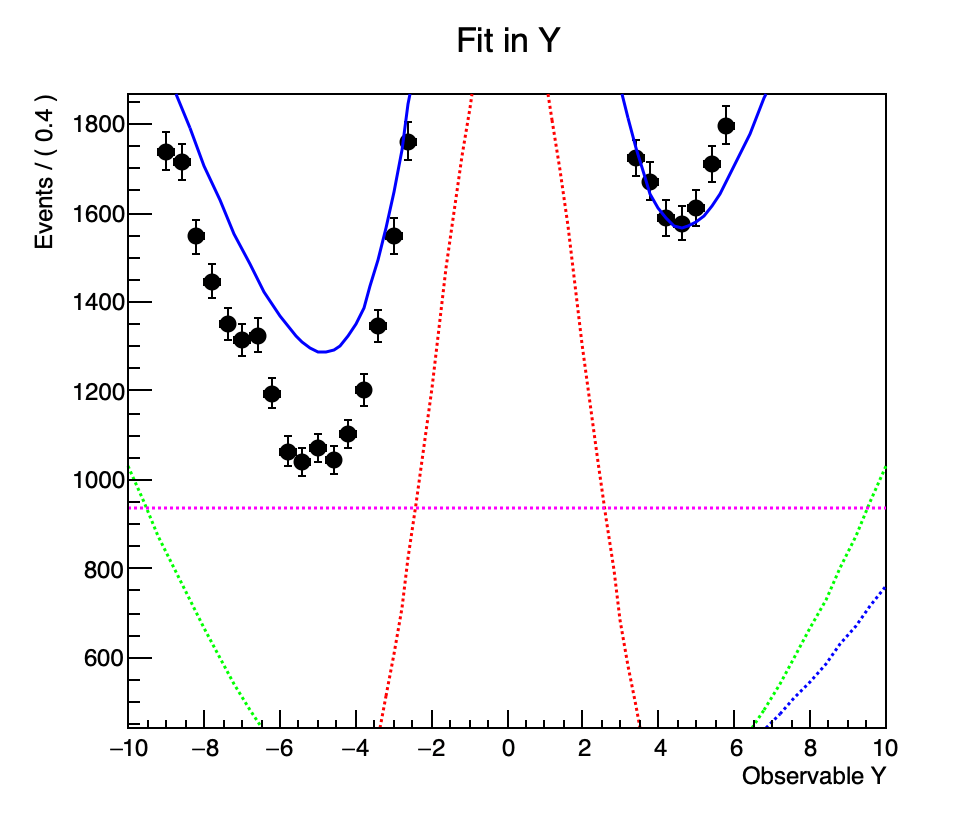
In the code example the projection on the y-Axis from the original background 3 histogram forms a flat line at 1000 entries per bin, while in the fitted model the (background3) component forms a line at about 937.

Here are the relevant lines:

// Signal: gaus in x and y
RooRealVar mean_x("mean_x", "Mean of X", 2, -5, 5);
RooRealVar sigma_x("sigma_x", "Sigma of X", 1, 0.1, 5);
RooGaussian gauss_x("gauss_x", "Signal Gaussian X", x, mean_x, sigma_x);
RooRealVar mean_y("mean_y", "Mean of Y", 0, -5, 5);
RooRealVar sigma_y("sigma_y", "Sigma of Y", 2, 0.1, 5);
RooGaussian gauss_y("gauss_y", "Signal Gaussian Y", y, mean_y, sigma_y);
RooProdPdf signal("signal", "Signal PDF", RooArgList(gauss_x, gauss_y));

// Background 1: exponential in x, 1st-order polynomial in y
RooRealVar bg1_x_tau("bg1_x_tau", "Tau parameter", -0.2, -5., -0.01);
RooExponential bg1_x_expo("bg1_x_expo", "Exponential in X", x, bg1_x_tau);
RooRealVar bg1_y_p0("bg1_y_p0", "Constant term in Y", 0);
RooRealVar bg1_y_p1("bg1_y_p1", "Linear term in Y", 0.1, -1, 1);
RooPolynomial bg1_y_poly("bg1_y_poly", "Polynomial in Y", y, RooArgList(bg1_y_p0, bg1_y_p1));
RooProdPdf background1("background1", "Background 1 PDF", RooArgList(bg1_x_expo, bg1_y_poly));

// Background 2: flat in x, 2nd-order polynomial in y
RooRealVar bg2_x_c0("bg2_x_c0", "Flat in X", 0);
RooPolynomial bg2_x_flat("bg2_x_flat", "Flat Polynomial in X", x, RooArgList(bg2_x_c0));
RooRealVar bg2_y_p1("bg2_y_p1", "Linear term", 0.1, -1, 1);
RooRealVar bg2_y_p2("bg2_y_p2", "Quadratic term", 0.01, -0.5, 0.5);
RooPolynomial bg2_y_poly("bg2_y_poly", "2nd order Polynomial in Y", y, RooArgList(bg2_y_p1, bg2_y_p2));
RooProdPdf background2("background2", "Background 2 PDF", RooArgList(bg2_x_flat, bg2_y_poly));

// Set yields for signal and backgrounds
RooRealVar nsig("nsig", "Number of signal events", 30000, 0, 100000);
RooRealVar nbkg1("nbkg1", "Number of background1 events", 30000, 0, 100000);
RooRealVar nbkg2("nbkg2", "Number of background2 events", 40000, 0, 100000);

// Model without background 3
RooAddPdf model_woBG3("model", "Total Model", RooArgList(signal, background1, background2), RooArgList(nsig, nbkg1, nbkg2));
// Generate a toy dataset
RooDataSet* data = model_woBG3.generate(RooArgSet(x, y), 100000);

// Add background 3 after data set generation (flat in x and y)
TH2* bg3_hist = new TH2F("bg3_hist", "Background 3 Histogram", 50, -10, 10, 50, -10, 10);
for (int i = 0; i < bg3_hist->GetNbinsX(); ++i) {
    for (int j = 0; j < bg3_hist->GetNbinsY(); ++j) {
        for (int k = 0; k < 20; ++k) {
            bg3_hist->Fill(bg3_hist->GetXaxis()->GetBinCenter(i + 1), bg3_hist->GetYaxis()->GetBinCenter(j + 1));
        }
    }
}
// Create DataHist and PDF for background 3 and set it to be constant
RooDataHist bg3_data("bg3_data", "Background 3 Data", RooArgSet(x, y), bg3_hist);
RooHistPdf background3("background3", "Background 3 PDF", RooArgList(x, y), bg3_data);
RooConstVar nbkg3("nbkg3", "Number of background3 events", bg3_hist->GetEntries());
// RooRealVar nbkg3("nbkg3", "Number of background3 events", bg3_hist->GetEntries());
// nbkg3.setConstant(true);

// Model with background 3
RooAddPdf model("model", "Total Model", RooArgList(signal, background1, background2, background3), RooArgList(nsig, nbkg1, nbkg2, nbkg3));

// Fit model with background 3 to data
RooFitResult* fitResult = model.fitTo(*data);

I also tried using a RooRealVar and setting .setConstant(true), but the issue persisted.

Is there a silly mistake on my side?
I’ve included a working example if anyone would like to try to reproduce the issue.

Any insights, suggestions, or corrections are highly appreciated!
Thanks

Fit2DConstant.cpp (5.4 KB)

[bellenot]

First, welcome to the ROOT Forum!
Then, I’m sure @jonas can help

[jonas]

Hi @fROOTtinator, cool user name!

This is just a plotting phenomenon (see RooAbsReal::plotOn).

If you plot a RooAbsPdf together with a RooDataSet, it will be automatically scaled to the sum of entries in the dataset. In your example, the total expected events in the model after the fit doesn’t exactly match with the sum of entries, so the scaling explains the phenomenon you see.

Let’s add some printouts around the fitting section in your script to understand what is going on:

    // Fit model with background 3 to data
    std::cout << "nbkg3          : " << nbkg3.getVal() << std::endl;
    std::cout << "dataset entries: " << data->sumEntries() << std::endl;
    RooArgSet nset{x, y};
    double expectedBefore = model.expectedEvents(&nset);
    std::cout << "expected before: " << expectedBefore << std::endl;
    RooFitResult* fitResult = model.fitTo(*data, Save(), PrintLevel(-1), PrintEvalErrors(-1));
    double expectedAfter = model.expectedEvents(&nset);
    std::cout << "expected after : " << expectedAfter << std::endl;
    fitResult->Print("v");
    delete fitResult;

The output:

nbkg3          : 50000
dataset entries: 100000
expected before: 150000
[#1] INFO:Fitting -- ...
expected after : 106661

Since even after the fit the expected number doesn’t match exactly the dataset, the backround3 value per bin is actually \frac{100000}{106661}\times 1000= 937.553, which is what you see.

If you want to undo this correction, then you can maybe add a relative normalization argument to your plotOn calls:

    RooCmdArg normArg = Normalization(expectedAfter / data->numEntries());
    // add this arg to the plotOn calls, like (model.plotOn(..., normArg))

In case you wonder why the post fit expected events doesn’t match the data, even though you were actually fitting it to data: by fixing the normalization of one of the components and not letting all of them float, you are introducing a correlation between shape and normalization. Therefore, statistical fluctuations in the shape of your toy dataset bias the post-fit expected number of events.

I hope this helps!

Cheers,
Jonas

[jonas]

Actually, I don’t think the default behavior of scaling extended pdfs to the number of observed events in the plot is of any use. I suggest we change it:

• [RF] Plotting extended pdf together with data unexpectedly scales pdf to number of events in data · Issue #18929 · root-project/root · GitHub

Would you agree with that?

[fROOTtinator]

Hi Jonas,

Thanks a lot for the quick reply and for the great explanation along with the suggestion how to bypass this correction. I’m not sure how much my opinion matters here, but as far as I’m concerned, I’m fine with making the change :).

Best Regards,
Adrian (fROOTinator)

[fROOTtinator]

Hi Experts,

Apologies for the follow-up question, and thanks in advance for your time.

I’ve been experimenting with the workaround using RooCmdArg normArg = Normalization(expectedAfter / data->numEntries()); applied to the dataset I actually want to fit. In this setup, I use projections from a TH3D and perform several preprocessing steps—such as adding and scaling histograms—before fitting.

To better illustrate the issue, I’ve prepared a minimal working example:
histograms.root (2.7 MB)
Fit2DConstant_Example2.cpp (9.1 KB)

The x-axis projections of the data (black) and the constant background (red, background 1 in the example) before the fit look like this:

Here are the expected event yields:
Before: 76740.5
After: 79364.2
So, a small correction is expected.

When I apply the relative normalization, the results looks like this:

For completeness and as a comparison, here’s the result without applying relative normalization:

My question is:
Could something in my preprocessing (projections, additions, scaling) be interfering with the relative normalization? Any suggestions are appreciated

Cheers,
Adrian

[jonas]

Hi, what is the reason for using RooAbsData::numEntries() and not RooAbsData::sumEntries(), like I suggested? For and unweighted RooDataSet, these are identical, but for a RooDataHist the numEntries() it returns the number of bins, which is not what you want here. Could that explain the wrong result?

Actually, the documentation is unclear on what numEntries() returns. I should also fix that up.

[fROOTtinator]

Hi Jonas,

I used numEntries() based on this comment:

@jonas

If you want to undo this correction, then you can maybe add a relative normalization argument to your plotOn calls:

    RooCmdArg normArg = Normalization(expectedAfter / data->numEntries());
    // add this arg to the plotOn calls, like (model.plotOn(..., normArg))

but I should have read this up in the documentation by myself. My bad…
Using sumEntries() seems to do the job for the constant background component (red component). This component now has the expected constant yield compared to the data.

But the total model (blue) including the other signal and background components with applied relative normalization does not match with the data anymore and is to high:

This makes sense to me, as normalization done after the fitting.
The second plot demonstrates the difference between models without relative normalization and with relative normalization. The shape of course does not change by the relative normalization.

Now the question: Is there a way to include the normalization in the fitting process, i.e that the model is fitted with initial yield of the constant background?
Another solution would be to just subtract the constant background from the data, but I would like to keep it in the fit if possible…

Cheers,
Adrian