You can obtain the values of the initial distribution like the sigma, µ and amplitude, but you cannot get the initial data before the smearing.
Below you find a code to find the initial values.
The codes use the convolution of the initial distribution with the gaussian for the resolution, and I use the convolution function created with TF1Convolution to fit the smeared data.
There is another example here
void macro()
{


    auto h1 = new TH1D("h1_gaus","Mass (amu);Counts",101.0,39.5,140.5);
    auto h1_smeared = new TH1D("h1_gaus_smeared","Mass (amu);Counts",101.0,39.5,140.5);
    double amu=0;
    for(long int i=0;i<320000;i++)
    {
        //generate the original data µ=87.5, sigma 12.86
        amu=gRandom->Gaus(87.52,12.86);
        //fill the histo with the original distribution
        h1->Fill( amu );
        //fill the histo with the smeared distribution
        h1_smeared->Fill( amu + gRandom->Gaus(0,3.5));
    }

    //define a TF1Convolution, note that the range is slightly larger than the original one
   // the 2 functions are both gaussians, the first is your original distribution while the latter is
  // for the resolution
    TF1Convolution *f_conv = new TF1Convolution("gaus", "gaus", 30.,150., true);

    f_conv->SetRange(30.,150.);
    f_conv->SetNofPointsFFT(1000);
    //I create a TF1 from the TF1Convolution
    TF1 *f = new TF1("f", *f_conv, 40., 140., f_conv->GetNpar());
    //I create a gaussian for the unsmeared distribution
    TF1 *f_gaus = new TF1("f_gaus_original","gaus", 40., 140.);

    // I set reasonable parameters for the convoluted function
    f->SetParameters(1e4,90.,13., 0.,3.5);
    // I fix the mean and the sigma of the gaussian accounting for the resolution
    f->FixParameter(3,0.);
    f->FixParameter(4,3.5);

    TCanvas *c = new TCanvas("c","c",800,1000);
    c->Divide(1,2);
    //I draw the original histogram in the top part
    c->cd(1);
    h1->Draw();
     //I draw the smeared histogram in the bottom part
    c->cd(2);
    h1_smeared->Draw();
   // I fit the smeared histogram with the convolution function
    h1_smeared->Fit(f);


    c->cd(1);
    //I use the parameters of the convoluted function found with the fit to initialize the value of the original gaussina
    f_gaus->SetParameters(f->GetParameters());
    double convoluted_gauss_area= 3.5*TMath::Sqrt(2*TMath::Pi());
    //I need to rescale the amplitude parameter with the area of the convolution function
    //This is due the math property of convolution
    f_gaus->SetParameter(0,convoluted_gauss_area*f_gaus->GetParameter(0));
   // Here I just draw the gaussian on the original histogram, I not use any fit
    f_gaus->Draw("same");

}
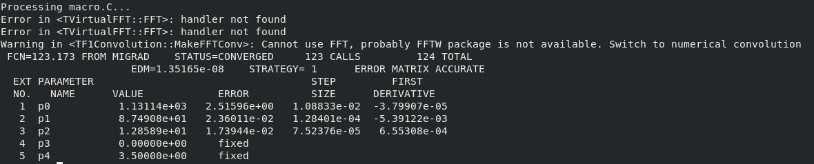
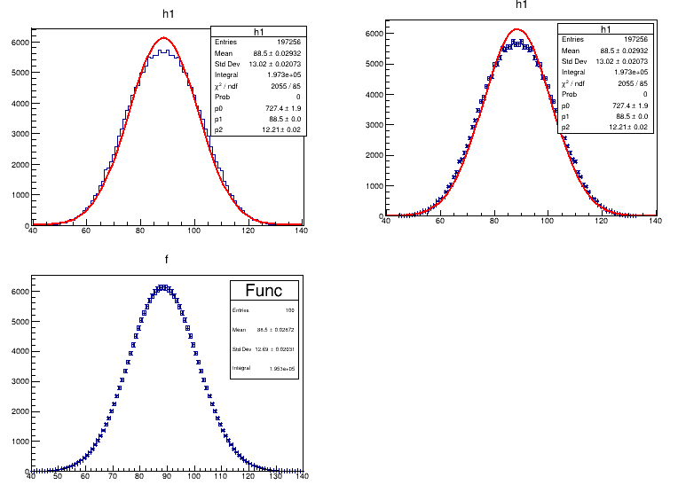
Here you found the results of the fit obtained with the convolution function
As you can see p1 (µ) and p2(sigma) are very close to the one I used to fill the initial histogram (µ=87.52, sigma= 12.86). Note also as p3 and p4 are fixed.
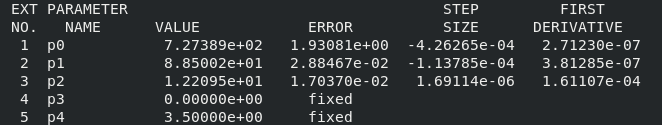
FCN=123.174 FROM MIGRAD    STATUS=CONVERGED     123 CALLS         124 TOTAL
                     EDM=2.30469e-09    STRATEGY= 1      ERROR MATRIX ACCURATE
  EXT PARAMETER                                   STEP         FIRST
  NO.   NAME      VALUE            ERROR          SIZE      DERIVATIVE
   1  p0           1.13228e+03   2.51851e+00   1.08943e-02   6.24005e-06
   2  p1           8.75508e+01   2.36011e-02   1.28403e-04  -2.38911e-03
   3  p2           1.28588e+01   1.73945e-02   7.52388e-05   2.55143e-03
   4  p3           0.00000e+00     fixed
   5  p4           3.50000e+00     fixed
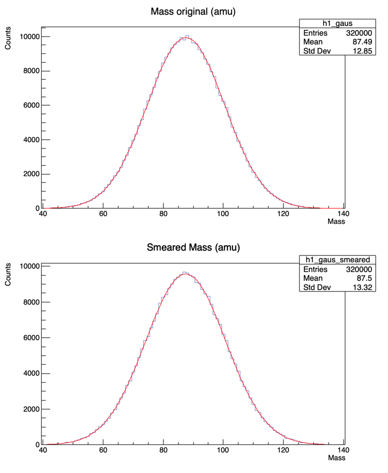
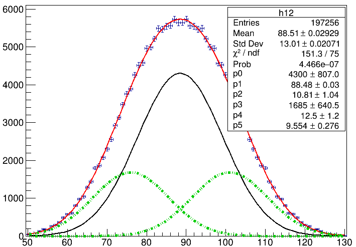
Here the plot obtained.