Obtaining the likelihood function after fitting

[Lepton86]

Dear ROOTers,

How does one obtain the likelihood function after fitting in RooFit?

If it’s a Gaussian likelihood G1(N, sigma_N), I want smear it by another Gaussian G2(N, sigma_P), where sigma_P describes some systematic or nuisance parameter. Specifically I want the convolution G1xG2.

I’m trying to find a more direct way to do what was suggested in these posts by @Stephan

Manipulate the likelihood

Hi all, to determine a significance, I compare the NLL differences for both, my nominal model and a null hypothesis (i.e. the nominal model with N_sig forced to be zero). Unfortunately, this only includes the uncertainties from the fit itself (statistical uncertaintes). I now want to determine a significance, where both uncertainties are included, the statistical and systematic one. What I read is that this could be accomplished by convoluting the likelihood with a Gaussian function, with the w…

Follow up on previous "Manipulate the likelihood" post

Hi @Lepton86, The sigScaler scales the amount of signal events (it’s multiplicative). When you use (... 1, 0, 2), the scale factor is initialised to 1, and allowed to vary within [0, 2]. The total signal then is nSig_scaled = sigScaler * nsig When initialised to 1, that’s obviously the model where no changes are happening. If the fitter decides that the sigScaler has to be changed to a value higher or lower than 1, a systematic uncertainty starts to have an effect on the fit. Here, the min …

In other words. Is there another way to include the systematics in the fit and thus significance in RooFit, or maybe specifically in RooStats?

Thank you.

[Lepton86]

Just to clarify, I ultimately want to do something like what’s asked about in this older post.

Convolution with a RooProfileLL

Hi, I have prepared a profile likelihood in the following way: RooNLLVar NLL("NLL","NLL",FinalPDF,*Data,Extended(true),ConditionalObservables(RooArgSet(*cond_var))); RooProfileLL PNLL("PNLL","PNLL",NLL,*N_Sig); RooAbsReal *profile_N_sig = PNLL.createProfile(*N_Sig); I can plot this simply by using: RooPlot *xframe = N_Sig->frame(); profile_N_sig->plotOn(xframe); And it gives the desired behavior. What I’d like to know is if there is a way to now convolve the plotted cur…

I meant to tag @StephanH originally and not the other person (sorry).

[StephanH]

Hi,

I’m not sure convoluting likelihoods is the right thing to do, but please find some more answers below.

@Lepton86

How does one obtain the likelihood function after fitting in RooFit?

With RooAbsPdf::createNLL(), e.g. like this:

auto nll = myFitModel->createNLL(data);

@Lepton86

If it’s a Gaussian likelihood G1(N, sigma_N), I want smear it by another Gaussian G2(N, sigma_P), where sigma_P describes some systematic or nuisance parameter. Specifically I want the convolution G1xG2.

In the posts you mentioned, I don’t see why likelihoods should be convoluted. You can convolute probability distributions, which yields the probability distribution of the sum of random variables, but I don’t think that this is what you are after.
Could you explain why you want to convolute?

@Lepton86

In other words. Is there another way to include the systematics in the fit and thus significance in RooFit, or maybe specifically in RooStats?

Yes, the standard way:

1. Find a parameter in the likelihood model that should “have” a systematic uncertainty.
   1.1 If the likelihood model doesn’t have such a parameter, introduce it. If you e.g. want the cross section of the signal process to vary within theory uncertainties, you replace xsec --> xsec * theoryUnc.
2. Multiply (don’t convolute) the likelihood function with a constraint term (= a PDF) that signifies how large the uncertainty is.
   If you e.g. want 10% theory uncertainty, you use

L(data | theoryUnc, <parameters ...>) =
  L(data | theoryUnc, <parameters ...>)_unconstrained
  * Gauss(1 | theoryUnc, 0.1)

Now, your theoryUnc can vary around 1 with a 1-sigma uncertainty of 10%. The trick is that the parameter shows up both in the “plain” likelihood as well as in the constraint term. If it only shows up in the former, it’s an unconstrained uncertainty. If it doesn’t show up at all (or if you set it constant), the systematic is switched off.

[Lepton86]

Hi Stephan,

Thanks for replying.

With RooAbsPdf::createNLL(), e.g. like this:

Yes, I got that after making the original post.

Could you explain why you want to convolute?

Yes. Basically it’s similar to the reason as in Manipulate the likelihood.

I am fitting for Nsig and I have some additional systematics I want to include that would have the effect of broadening the profile curve of Nsig, giving me larger asymmetric errors than without the systematics included. I have tried the method in that prior post but for me it only works some of the time. Some of the time it fails. So I want to know if there’s a direct way to do it without introducing a new nuisance parameter, e.g. bu directly manipulating the input NLL by adding information about the systematics to it.

Now, your theoryUnc can vary around 1 with a 1-sigma uncertainty of 10%. The trick is that the parameter shows up both in the “plain” likelihood as well as in the constraint term. If it only shows up in the former, it’s an unconstrained uncertainty. If it doesn’t show up at all (or if you set it constant), the systematic is switched off.

Please correct me if I’m wrong but wouldn’t this have the effect of narrowing the profile LL instead of broadening it. What you suggest is what I originally thought but my goal isn’t to “constrain” my parameter of interest Nsig1, which would make the errors smaller. I want the opposite effect after including the systematics. I want to smear the profile LL including the systematics on the profiled parameter (Nsig) into the likelihood function.

So I want to convolve the original likelihood of my parameter of interest L1(Nsig | mu, sigma1) with a Gaussian centered at zero L2(Nsig | 0, sigma2) where sigma2 are is the systematic associated with Nsig thus giving a widened profile curve than the original.

After making this post I tried doing it manually a couple of ways, for example taking the sum of the NLL instead of convolving the LL.

nll = model.createNLL(data, ROOT.RooFit.Extended()) # -Log(L1)

nll2 = TF1("fconstraint2","-TMath::Log(TMath::Gaus(x,[0],[1],0))", NsigLO, NsigHI)

nll2_bind = ROOT.RooFit.bindFunction(nll2, nsig)

total_nll = ROOT.RooAddition("total_nll", "total_nll", ROOT.RooArgList(nll, nll2_bind))

Then create the profile from total_nll.

But I don’t think this is exactly right. Any suggestions you could give on this problem would be greatly appreciated.

Just a quick update. I tried the following method, going off my idea above:

        # manually create the NLL from a Gaussian defined by absolute uncertainties
        syst_nll = TF1("syst_nll","-TMath::Log(TMath::Gaus(x,[0],[1],0))", sigLO, sigHI)
        syst_nll.SetParameters(0, syst_uncert) # parameterize the NLL for the systematics here
        
        # make TF1 a RooAbsReal
        syst_NLL_bind = ROOT.RooFit.bindFunction(syst_nll, nsig)
        
        # create NLL from original (unconvolved) fit
        nll = model.createNLL(data, ROOT.RooFit.Extended())
        
        # make original NLL a TF1 then a RooAbsReal
        nll_asTF = nll.asTF(ROOT.RooArgList(nsig)) 
        nll_rooabsreal = ROOT.RooFit.bindFunction(nll_asTF, nsig)
        
        # get original ("unconvolved") profile for comparison
        pll = nll_rooabsreal.createProfile(nsig)
        
        # add them together ("convolution")
        total_nll = ROOT.RooAddition("total_nll", "total_nll", ROOT.RooArgList(nll_rooabsreal, syst_NLL_bind))
        
        # minimuzation and other stuff
        minimize_total_nll = ROOT.RooMinimizer(total_nll)
        minimize_total_nll.minimize("Minuit", "Migrad")
        minimize_total_nll.hesse()
        minimize_total_nll.minos(nsig)
        total_pll = total_nll.createProfile(nsig)

	# plot (problem?  profiles seem exactly the same even though fit results are not)
        frame = nsig.frame()

        c1 = ROOT.TCanvas("myCanvas", "myCanvas", 1280*2, 1024*2)
        ROOT.gPad.SetLeftMargin(0.15)

        total_pll.plotOn(frame, ROOT.RooFit.LineColor(ROOT.kRed))
        frame.Draw()
        pll.plotOn(frame, ROOT.RooFit.LineColor(ROOT.kBlue))
        frame.Draw("SAME")
        c1.SaveAs("test.png")

Here is the fit result from before the “convolution”.

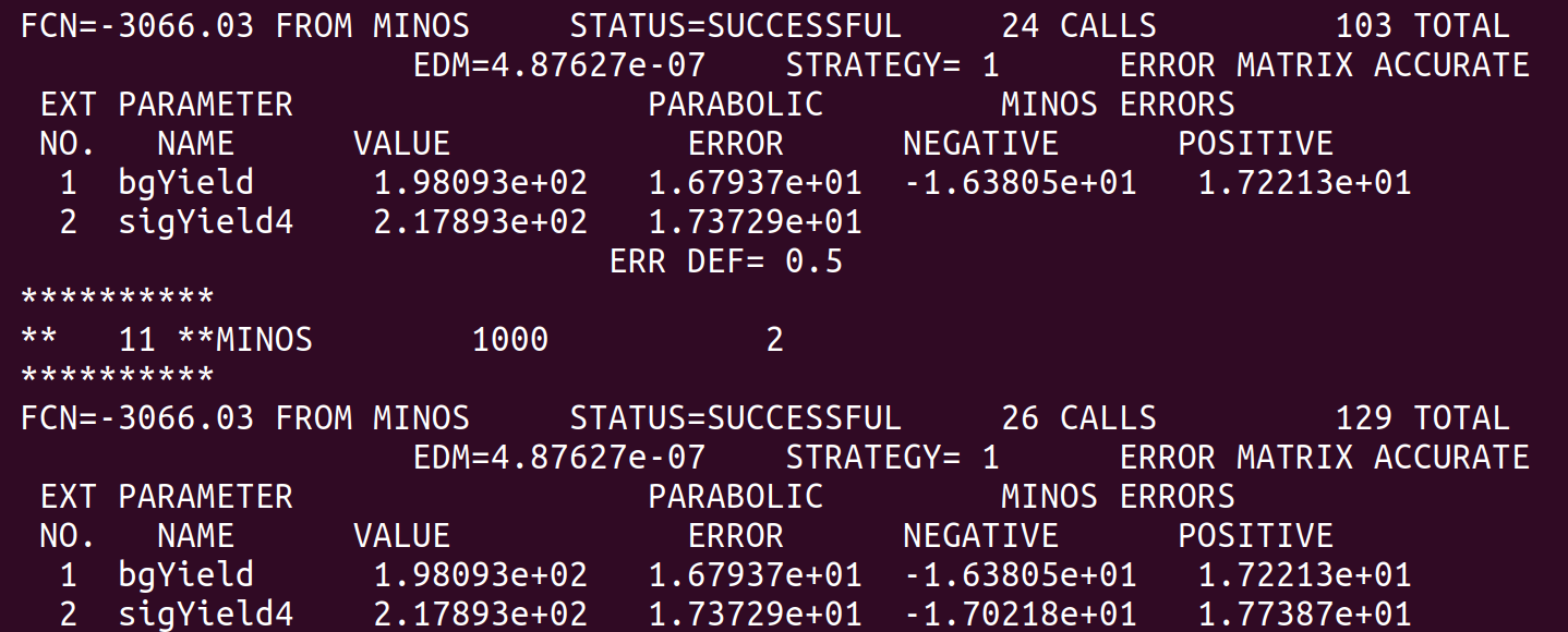
And here is the result after the convolution.

At least naively it does what I expect. The MINOS errors after the convolution are enlarged due to the addition of the systematics. However, this is only a small scale test and when I try to plot the profile on the same canvas they overlap exactly. See the following plot.

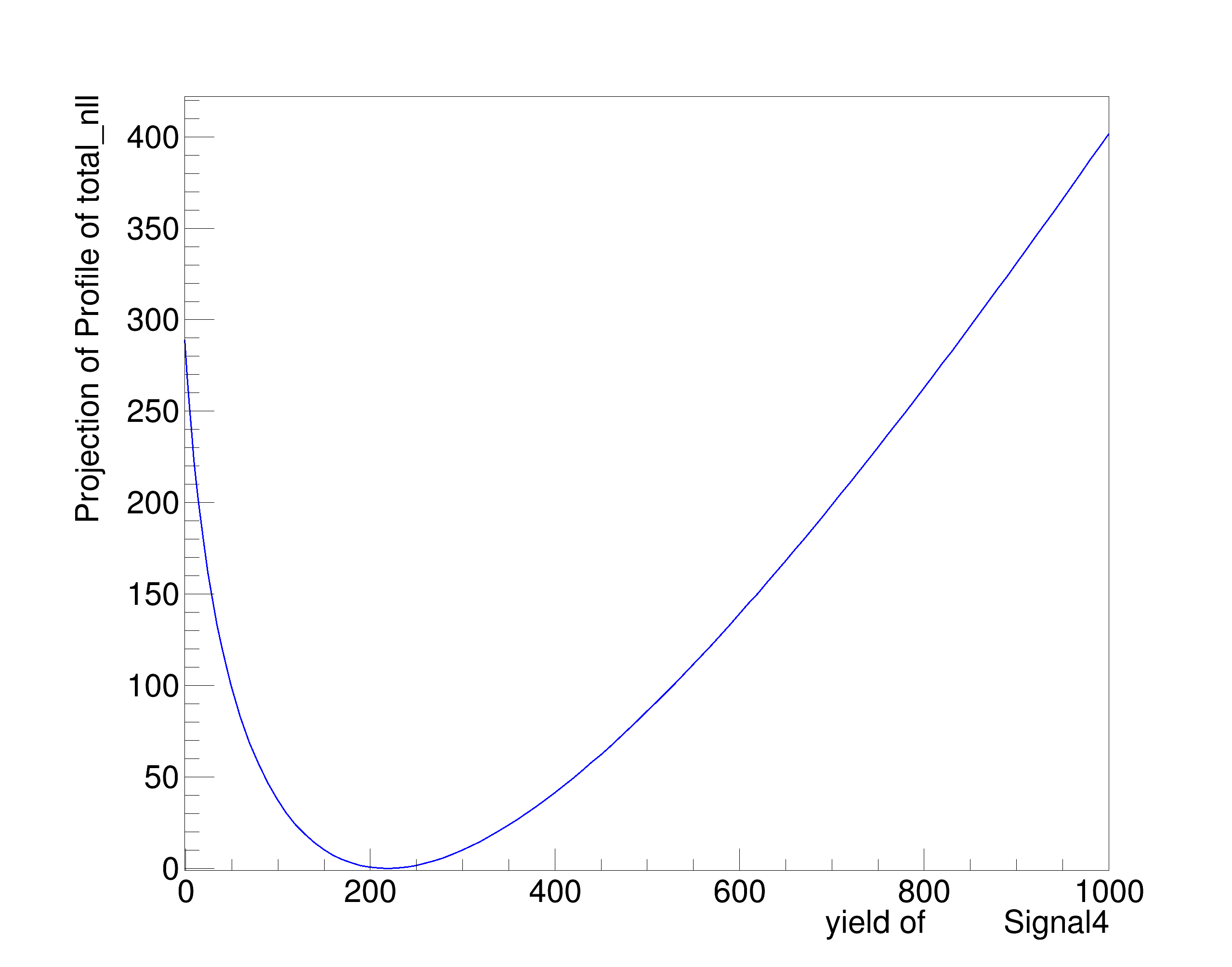
There should be red curve for before convolution and blue for after convolution but they overlap so it isn’t apparent is there is a difference. I’m not sure if this is due to a plotting error or I’m not actually getting the result I want as shown in the fit screen captures above.

[StephanH]

Hello,

Please find some answers below.

@Lepton86

Please correct me if I’m wrong but wouldn’t this have the effect of narrowing the profile LL instead of broadening it. What you suggest is what I originally thought but my goal isn’t to “constrain” my parameter of interest Nsig1 , which would make the errors smaller. I want the opposite effect after including the systematics. I want to smear the profile LL including the systematics on the profiled parameter ( Nsig ) into the likelihood function.

It’s true: constraining a parameter narrows the profile, but if you introduce a new nuisance parameter, the likelihood profile is broadened. In the most extreme case, if you introduced a parameter that is almost 100% correlated with your parameter of interest and in addition unconstrained, you would get infinitely large errors / an infinitely large likelihood profile.
By the way: If you add a signal scale factor, it’s -100% correlated, and will completely destroy any sensitivity that you fit model has. Only if you constrain it, you can get reasonable results, and if you make the constraint infinitely strong, it’s like the parameter never existed.

I really don’t think that convoluting the NLL with some function is correct. Unless you can point me to some literature that explains why convolution can work, I assume that you won’t get the desired result if you use a convolution.

@Lepton86

But I don’t think this is exactly right. Any suggestions you could give on this problem would be greatly appreciated.

I checked the code snippets that you posted, but there’s no convolution anywhere. I only see additions. Additions of the log-likelihood, however, are multiplications of the likelihood. This would be the “standard” way to introduce (and constrain) a systematic uncertainty.

The way it’s done in those snippets, it’s more complicated, though. If you write it in the “normal” way, it should look something like this:

syst_nll = ROOT.RooGaussian("syst_nll", "...", centralValue, systParameter, uncertainty)
totalL = ROOT.RooProdPdf(..., ..., ROOT.RooArgList(model, syst_nll) )
total_nll = totalL.createNLL(data)

Note also that a Gaussian distribution with Gaus(x, sigLo, sigHi) does not vary between lo and hi. It is a distribution with central value sigLo, and width (sigma) of sigHi.

@Lepton86

At least naively it does what I expect. The MINOS errors after the convolution are enlarged due to the addition of the systematics.

I think this is completely wrong, but please correct me if I’m missing something. In the second case, where errors seem to be larger, bgYield somehow disappeared from the model, so it’s doing something completely different.

I don’t know if I sent it already, but here’s the tutorial on how to introduce constraints:
https://root.cern/doc/master/rf604__constraints_8C.html

@Lepton86

There should be red curve for before convolution and blue for after convolution but they overlap so it isn’t apparent is there is a difference.

You would see a drastic difference if the systematic had any effect. This cannot be correct.

[StephanH]

@Lepton86

I will try to find something to demonstrate what I mean. But for now all I want to do is smear the resultant profile likelihood in sigYield, not constrain it (even if it is not mathematically well defined). That’s what I’m trying to figure out how to do in RooFit.

I see. The reason there’s no obvious way to do it is probably that it’s not well defined.

@Lepton86

It is not explicitly a convolution, it’s just a way to introduce the systematics to make the profile wider. The high error should then naively be approximately sqrt(stat. err^2 + syst. err^2), where the stat err is the error from the normal fit. That’s what I’m ultimately trying to get to.

If stat error and systematic error are sufficiently uncorrelated, that’s what you will get when you introduce the systematic in the “standard way”.

@Lepton86

Yes. Did I make that mistake somewhere?

Yes, here:

@Lepton86

syst_nll = TF1("syst_nll","-TMath::Log(TMath::Gaus(x,[0],[1],0))", sigLO, sigHI)

@Lepton86

I’ve tried that. But that constrains (narrows) the profile of the POI, unless I misunderstood something.

No, no misunderstanding. It is supposed to narrow it. Let me reiterate:

• Introduce a nuisance parameter → Profile widens (but maybe more than you want, because the effect is unconstrained.
• Introduce a nuisance parameter + constrain it → Profile widens, but by the “correct” amount.
• Introduce a nuisance parameter + constrain it infinitely strongly → Profile remains the same as if you didn’t introduce the NP.

@Lepton86

The nuisance parameter ( sigScaler in your solution) can vary such that the profile is not at all parabolic and the high MINOS error is much larger than the approximation sqrt(stat. err^2 + syst. error^2). For example.

Corresponding to the fit result

But that’s exactly right! If you introduce the nuisance parameter, and don’t constrain it, your errors will explode! You basically say: The signal systematic can be as strong as the fitter desires, even infinitely strong. Here, you completed step 1 so to say.

@Lepton86

If I set the lower bound on sigScalar to be higher than zero, e.g. 0.5, I get a more parabolic profile and the error is closer to what I expect, but MINOS gives the “at limit” warning.

The range of the parameters should not be used as constraints. They are really hard limits, which convey physical limits (e.g. that a signal scaler cannot be negative). What’s missing now is that you say:
“The signal scaler is allowed to vary between 0.8 and 1.2” (or whatever is appropriate for your systematic). This is what you do by additionally introducing a constraint on the nuisance parameter.

Again:

• Adding a NP increases errors. You did that.
• Constraining the NP will get it to the “right amount”.

[Lepton86]

@StephanH, I understand the reasoning behind your additional NP method better. Thank you. Just a couple of minor points to clarify then I think that should be it.

@StephanH

Yes, here:

[quote="Lepton86, post:4, topic:40910"]
`syst_nll = TF1("syst_nll","-TMath::Log(TMath::Gaus(x,[0],[1],0))", sigLO, sigHI)`
[/quote]

I followed this ROOT: TF1 Class Reference. I then used SetParameters(...) to set the formula parameters. When I plot it I get what I expect but I’ll check again. I probably overlooked something.

@StephanH

If stat error and systematic error are sufficiently uncorrelated, that’s what you will get when you introduce the systematic in the “standard way”.

I used your sketch of the standard way.

        syst_nll_mean = ROOT.RooRealVar("syst_nll_mean", "syst nll gaussian mean", nsig_val)
        syst_nll_sigma = ROOT.RooRealVar("syst_nll_sigma", "syst nll gaussian sigma", syst_uncert)
        syst_nll = ROOT.RooGaussian("syst_nll", "syst_nll_gaus", nsig, syst_nll_mean, syst_nll_sigma)
        totalL = ROOT.RooProdPdf("totalL", "totalL", ROOT.RooArgList(model, syst_nll))
        total_nll = totalL.createNLL(data)
        minimize_total_nll = ROOT.RooMinimizer(total_nll)
        minimize_total_nll.minimize("Minuit", "Migrad")
        minimize_total_nll.hesse()
        minimize_total_nll.minos(nsig)

If I didn’t make a mistake, you say that the new error should be sqrt(stat. err^2 + syst. err^2), if the errors are uncorrelated. That would make the new error larger. But I seem to get smaller errors?

@StephanH

No, no misunderstanding. It is supposed to narrow it. Let me reiterate:

• Introduce a nuisance parameter → Profile widens (but maybe more than you want, because the effect is unconstrained.
• Introduce a nuisance parameter + constrain it → Profile widens, but by the “correct” amount.
• Introduce a nuisance parameter + constrain it infinitely strongly → Profile remains the same as if you didn’t introduce the NP.

Thanks for this, I understand it better now.

@StephanH

The range of the parameters should not be used as constraints. They are really hard limits, which convey physical limits (e.g. that a signal scaler cannot be negative).

To clarify, I meant that the “at limit” warning was for the sigScalar

@StephanH

What’s missing now is that you say:
“The signal scaler is allowed to vary between 0.8 and 1.2” (or whatever is appropriate for your systematic). This is what you do by additionally introducing a constraint on the nuisance parameter.

Again:

• Adding a NP increases errors. You did that.
• Constraining the NP will get it to the “right amount”.

Then is my understanding correct, on a practical level, that when I constrain the NP to the “right amount” (i.e. set the bounds on the NP based on what I think corresponds to the physics) that the “at limit” message from the fitter is ok if the fit is successful and I get “sensible” asymmetric errors? I think this practical usage of RooFit is what concerns me the most, with respect to this problem.

[StephanH]

@Lepton86

When I plot it I get what I expect but I’ll check again. I probably overlooked something.

Here you set sigLo as the mean, and sigHigh as the sigma. That likely not what you wanted.

@Lepton86

If I didn’t make a mistake, you say that the new error should be sqrt(stat. err^2 + syst. err^2), if the errors are uncorrelated. That would make the new error larger. But I seem to get smaller errors?

You have to compare error with NP and error with NP+constraint. The former should be a lot larger, the latter a bit larger than the model without NPs.

@Lepton86

To clarify, I meant that the “at limit” warning was for the sigScalar

Yes, that’s what I understood. However, (see below), you should not use the range of a parameter to constrain it. It’s more like a safety check that the normalisation doesn’t go negative. Once you see those warnings, something is already going wrong. (When this happens, you don’t get an NLL “parabola”, but it’s like an infinitely large wall that the minimiser cannot jump over. You will get wrong errors when Minos hits it.)

@Lepton86

Then is my understanding correct, on a practical level, that when I constrain the NP to the “right amount” (i.e. set the bounds on the NP based on what I think corresponds to the physics) that the “at limit” message from the fitter is ok if the fit is successful and I get “sensible” asymmetric errors? I think this practical usage of RooFit is what concerns me the most, with respect to this problem.

No, you need to set the errors a bit differently. Let’s say you want a 10% signal uncertainty. What you do is to add a signal scale factor, and you give it a range of something like [0, 2].

syst_np = ROOT.RooRealVar("syst_np", "...", 1, 0, 2) #Start at 1, and go between 0 and 2 before hitting the wall
syst_nll_mean = ROOT.RooConstVar("NP_central", "Central value of constraint", 1)
syst_nll_sigma = ROOT.RooConstVar("NP_sigma", "Uncertainty of constraint", 0.1)
constraint = ROOT.RooGaussian(.., .., syst_nll_mean, signalScaler, syst_nll_sigma).

The sigma of 0.1 in the Gaussian distribution is the systematic uncertainty. The allowed range of the signal scaler should be much larger than that! In this case I set it to [0, 2], that’s 10 sigma away from its central value.
NB: RooConstVar is a shortcut for a constant value, roughly equivalent to a RooRealVar that you set to constant.

To convince yourself that the systematic is working correctly, run the following test:

• Set the sigma to something like 10 or 100 times the original size. You should now get ridiculously large errors.
• Set it to the desired amount, e.g. 10%. You should now get errors that are more or less sqrt(stat^2 + sys^2)
• Set it to something really small, e.g. 0.00001%. Your error should now be virtually the same as the stat error. The systematic should be switched off.

If all three work out as expected, you implemented it in the right way. You can obviously also test 2*systUncertainty, and expect roughly sqrt(stat^2 + 4 * syst^2) if you want to get a feeling of the impact.

Also note that if you want to “switch off” the systematic uncertainty, you can simply use sigScaler.setConstant(True). Use this after you made sure that it’s implemented correctly. This is handy if you want to break down the total error in single components. You “switch off” the impact of one component, and measure the total error. That tells you how important the systematic is.

[Lepton86]

I may have spoken prematurely when I said there are only minor points to clarify but thanks for sticking with it thus far.

@StephanH

constraint = ROOT.RooGaussian(.., .., syst_nll_mean, signalScaler, syst_nll_sigma).

Your RooGaussian construction has the mean and signalScalar in different positions than I expect from the class reference. Is that right? And is syst_np = signalScaler?

@StephanH

To convince yourself that the systematic is working correctly, run the following test:

@StephanH

Set it to the desired amount, e.g. 10%. You should now get errors that are more or less sqrt(stat^2 + sys^2)

Yes this is what I get and the profile looks more or less correct at small scales of the POI.

@StephanH

Set it to something really small, e.g. 0.00001%. Your error should now be virtually the same as the stat error. The systematic should be switched off.

Also consistent with what I get.

@StephanH

Set the sigma to something like 10 or 100 times the original size. You should now get ridiculously large errors.

This is the troublesome part and where my understanding is not as good as to the practical implementation. To be clear, this is what I have.

signalScaler = ROOT.RooRealVar("signalScaler", "...", 1, 0, 2) # syst_np = signalScalar from above
syst_nll_mean = ROOT.RooConstVar("NP_central", "Central value of constraint", 1)
syst_nll_sigma = ROOT.RooConstVar("NP_sigma", "Uncertainty of constraint", 0.1)
constraint = ROOT.RooGaussian(.., .., signalScaler, syst_nll_mean, syst_nll_sigma) # signalScaler, syst_nll_mean swapped positions from above

nSig_scaled = ROOT.RooProduct("nSig_scaled", "nSig_scaled", ROOT.RooArgList(Nsig, signalScaler)) # the scaled signal yield

model = ROOT.RooAddPdf("model", "model", ROOT.RooArgList(sigPdf, bkgPdf), ROOT.RooArgList(nSig_scaled, Nbkg)) # total model is sum of signal+bkg PDF

constrained_model = ROOT.RooProdPdf("constrained_model", "constrained_model", ROOT.RooArgList(model, constraint)) # "constrain" the model

fitResult = constrained_model.fitTo(data, ROOT.RooFit.Minos(), ROOT.RooFit.Extended())

syst_nll_sigma is parameterized by the relative systematic uncertainty, e.g. if Nsig = 20 events (Nsig = POI to be profiled) and there is a 2 event uncertainty I want to include in the profile then syst_nll_sigma = 2/20 = 0.1. Please shout out if that’s the wrong understanding. If I make the error 10x larger, i.e. 100% of Nsig in this case, then the fitter throws the “at limit” warning and the profile looks exactly flat, when I want it to look more or less parabolic. However you said not to use the range of parameters as a constraint to fix the issue. That’s where my understanding breaks down.

I don’t mean this as an exercise to check the fitter, I mean what if I actually have an error that e.g. 200% of the central value? I should in principle still be able to include that in the profile, which should be parabolic, even if it might be very broad. The error should still be approximately sqrt(stat.^2 + syst.^2) but instead it seems to break down and the fitter can’t converge.

[StephanH]

@Lepton86

Your RooGaussian construction has the mean and signalScalar in different positions than I expect from the class reference. Is that right? And is syst_np = signalScaler ?

I like to think about the parameter as the mean, and the “global observable” as the observable, but the gaussian is symmetric in those two parameters because of the square. That is, you can interchange them.

@Lepton86

there is a 2 event uncertainty I want to include in the profile then syst_nll_sigma = 2/20 = 0.1 . Please shout out if that’s the wrong understanding. If I make the error 10x larger, i.e. 100% of Nsig in this case, then the fitter throws the “at limit” warning and the profile looks exactly flat, when I want it to look more or less parabolic.

That’s correct. The at limit warning happens because the sigScaler hits the limit of [0,2], and as I told you, that’s a hard limit. Everything seems to work as expected, so I think your fit model is done now.

However, if you need a 200% scale uncertainty, think about what that means for the amount of signal: -20 events. Does this make sense in your case? If yes, allow negative signal scale factors, e.g. [-5, 6] or so, and continue.
Some people, however, define scale systematics such that +N sigma for a 10% systematic is 1.1^N, and -N sigma is 0.9^N. In that case, you can also set the nuisance parameter to 10 sigma, and you will still not go below zero. Which of the two approaches you use is up to you.