Max likelihood fit with a TGraphAsymmErrors (basically how to do a unbinned likelihood fit)

[malfonsi79]

Dear ROOTers,

I would like to do a likelihood fit rather than a chisquare fit on the unbinned data with a TGraphAsymmErrors, but I have the impression that this is possible only with histograms.

I explain my problem, maybe I will get also some suggestion about the correct statistical treatment of my problem.

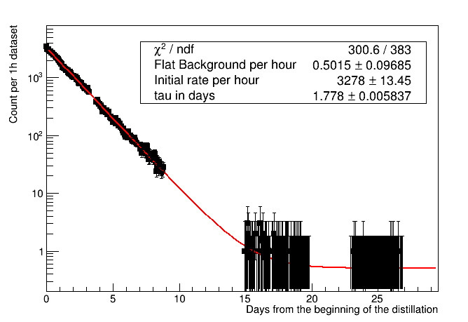
I want to fit the exponential reduction of activity counts over time, very simple (with some expected small flat background). I have datasets of about one hour, but not always contiguous (normally few minutes in between, but there are also few days gaps) and for each of them my selection gives me the counts within this hour. So the rate is the counts divided the “live time” of the dataset, with an error as the sqrt(counts) divided the livetime.
The problem comes from the last “measurement points”, where I get more and more 0 counts.

I do not see an option for max likelihood fit in TGraphAsymmErrors and chisquare fits cannot take into accounts zeros. Moreover already when I have few counts per datasets I would like to use the more accurate asymmetric “poisson” error.

So far my workaround is to group together datasets in days, but now I have the same problem in the last few days, and this is the period where I start to see a change of slope and I need to figure out if it is really a change of slope or a background larger than expected.

One solution could be to make a TH1D with variable bin size to place the measurement points at the center of each bin, but 1) I am not sure how this variable bin size enters into the likelihood 2) the few days gaps are either a wrong zero data points or they move the center of the adjacent bin if I decide to merge them to the next bin.

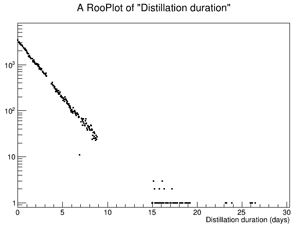
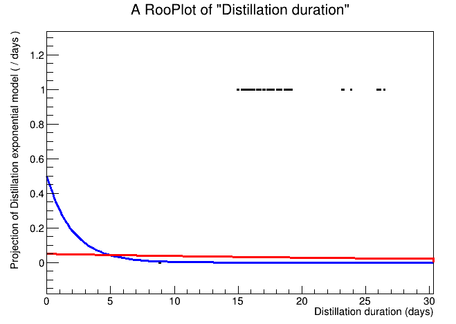
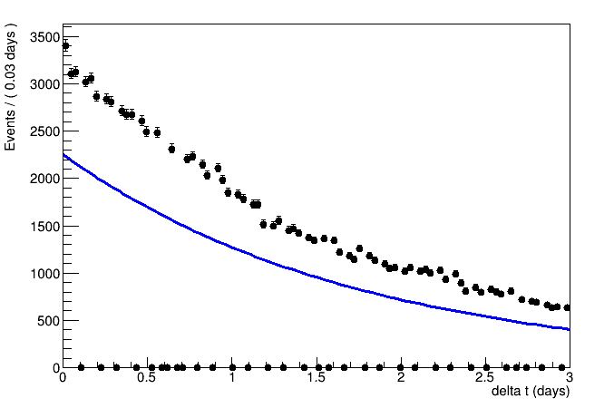
If there are no options with TH1 or TGraphAsymmError, I have quickly read that RooFit performs unbinned max likelihood fit and I wonder if this is the way to go (but I have to learn the tool…)

Any suggestion is very welcome,
Matteo

---

ROOT Version: 6.14/02 or master, but I doubt that this matters in this case
Platform: Debian 9
Compiler: gcc 6.3

---

[StephanH]

Hi @malfonsi79,

Do you record all counts directly, or do you only record the counts per hour? These things might get you started:

• In the first case, an unbinned fit is exactly what you need.
  $ROOTSYS/tutorials/roofit/rf102_dataimport.C (Tutorial website) shows some ways how to import unbinned data.

• In the second case, it also works with an unbinned fit, but we would have to change the weights of the events. There is also an example to do this,
  $ROOTSYS/tutorials/roofit/rf403_weightedevts.C, which you will also find on the (Tutorial website).

• tutorials/roofit/rf205_compplot.C shows how to use an exponential distribution in RooFit.

[malfonsi79]

Thanks,

so I guess that RooFit is the way to go.

I used to produce a text file with three columns:

1. start date (I used TDatime to plot on TGraph, but I can just change this to time from the beginning)
2. counts per dataset
3. duration (typically 1h ± few seconds, but some are shorter)

Maybe, to start with, I can use only files with the typical 1h duration (ignoring the few seconds jitter) and make a file with 2 columns:

1. start date
2. counts, that can be taken basically as rate per hour (instead of the rate per second as I used)

According to your links, I can just import the text file and RooFit calculate Poisson error by default, isn’t it?

In a later stage, if I want to use all also datasets of shorter duration, I should introduce weights to penalized them, following the procedure in your second link. But what is the right weight to use? Is it statistically right to say that counts observed for half the time should have a factor 2 penalty? (sorry if I ask about statistics rather than about RooFit)

Thanks again,
Matteo

[StephanH]

Hi Matteo,

the optimal weight is 60/minutes measured. That is, using the weight you convert each measurement to exactly one hour. Put this in a histogram, where the x-axis is in hours (or another time unit of your choosing), and fit it.
Make sure to use the SumW2 as shown in the 403 tutorial to obtain corrected errors. The deviations from true Poisson statistics should be very small if your intervals only deviate by seconds, but for the shorter intervals with high weights this is important.

[malfonsi79]

Dear Hageboeck,

I think that I am not using the tool in the right way.

The first picture shows what I would like to do with the TGraphAsymmErrors. I have also changed the error to poisson errors as it is done inside the TH1x classes, but since I am still doing a chi2 fit I think that the result is not correct, e.g. if I group together all the datasets belonging to the same day the flat background results much smaller.

With roofit I managed to import data and visualize them (after discovering that I should use plotOnXY rather than plotOn, because the latter forces some binning), but errors are not shown:

Moreover I am clearly doing wrong with the fit (for the moment I just use the exponential without constant background), because I do not understand how the “Y” axis, or the overall normalization if you want, should be introduced in the fit.

When I plot the model before fitting, with some reasonable initial value for the decay parameter, the function is plotted much more below 1, probably because it is normalized to 1, see the blue line below. Moreover I cannot plot it in log scale because I have complaints on some value below 0. After the fit (red line) the function become even worse, so it is clear that I am using roofit in the wrong way.

Can I have some more hint?

Thanks,
Matteo

[StephanH]

Hi Matteo,

It looks to me that you made a 2D plot, didn’t you? I would advise to make an unbinned dataset, but assign each measurement a weight according to the precision we can expect from the counts.

When plotting a 1D model, RooFit should automatically adjust the normalisation of the fitted PDF to the data if you first plot the data and then the model.

[malfonsi79]

Dear Hageboeck,
thanks again.

@StephanH

It looks to me that you made a 2D plot, didn’t you? I would advise to make an unbinned dataset, but assign each measurement a weight according to the precision we can expect from the counts.

Any my attempt to do a 1D plot, despite having a binned plot while all the point was to have something unbinned, seems to show just the distribution of times rather than bins filled as the second “counts” variable. With a ROOT TH1F, I would Fill(t, counts) using the counts variable as a “weight” for filling. How can I do that here?

An extract of my script (I restricted the time range to only the first 3 days where a model for background is not needed and the fit should be a really trivial exponential fit):

  RooRealVar deltat("deltat", "",1., 0., 3., "days");
  timeframe = deltat.frame();
  RooRealVar countsds("countsds", "counts per dataset", 10, 0., 1e5, "");
  //not used right now
  //RooRealVar livetimeds("livetimeds", "Livetime of the dataset", 3600, 0., 36000., "s");
  
  RooDataSet* mydata = RooDataSet::read("test.csv", RooArgList(deltat, countsds) );

  mydata->plotOn(timeframe,Binning(70))->Draw(); //makes no sense, it is the distribution of deltat
  mydata->plotOnXY(timeframe, YVar( countsds))->Draw() //this makes sense, but no error bars

@StephanH

When plotting a 1D model, RooFit should automatically adjust the normalisation of the fitted PDF to the data if you first plot the data and then the model.

I read on the manual about extended pdf and this seems the way to go to fit also the initial number of events:

  RooRealVar alpha("alpha","Exponential decay rate per day parameter",
		       -0.5,-10., 0.) ;
  RooExponential modelExpo("modelExpo","Exponential model", deltat,alpha) ;
  RooRealVar nsig("nsig","Signal event counts",500,0,10000.) ;
  RooExtendPdf modelSig("modelSig","Signal event counts model", modelExpo, nsig) ;

  auto res = = modelSig.fitTo( mydata, Save() )

but the result is just wrong, I think it is again fitting the distribution of times. Actually, in all this business I think that I have not found the way to tell roofit that the variable countsds (the second column of my text file) is the “Y variable” or the “bin content variable”, and indeed how can roofit guess this info, e.g. if in mydata there were 3 columns? So probably this is the missing piece that I do not get from the documentation.

Matteo

[StephanH]

To make the dataset weighted, you could do the following (from tutorial rf403):

//Your code
RooRealVar deltat("deltat", "",1., 0., 3., "days");
timeframe = deltat.frame();
RooRealVar countsds("countsds", "counts per dataset", 10, 0., 1e5, "");
RooDataSet* mydata = RooDataSet::read("test.csv", RooArgList(deltat, countsds) );

// Construct weighted set
// Construct formula to calculate weight for each event
RooFormulaVar wFunc("w", "event weight", "(countsds)", countsds) ;
// For now, the weight is just the measured number of events. However, this can be used to scale the counts 
// such that they correspond to counts per hour. E.g. "countsds * 60./livetimeds"

// Add column with weight
RooRealVar* w = (RooRealVar*) data->addColumn(wFunc) ;
data->Print() ;

// Instruct dataset wdata to interpret w as event weight rather than as observable
RooDataSet wdata(data->GetName(),data->GetTitle(),data,*data->get(),0,w->GetName()) ;
wdata.Print() ;

One piece of information that I’m missing, though:
Did you measure the counts for each interval? In that case, you have to adjust the weights to reflect this change, because a count that you measured N times is obviously better than a count that you measured only once.

[malfonsi79]

Dear Hageboeck,

thanks. This was the missing information, I thought that the weights were coming into play only when I had to apply the livetime corrections.

The fit now makes sense and I have other problems, but let me first answer to your question:

@StephanH

One piece of information that I’m missing, though:
Did you measure the counts for each interval? In that case, you have to adjust the weights to reflect this change, because a count that you measured N times is obviously better than a count that you measured only once.

My text file has three columns, each row represent the results of a selection on a single dataset:

1. start time of the dataset relative to the very first dataset.
2. the number of the events passing selection (it can be interpreted as counts/hour since the typical duration of the dataset is 1h)
3. effective duration of the dataset, representing the effective observation time once that DAQ busy or fraction of time with other problems are removed. But for the moment let’s ignore this part.

0.0 3402.0 3603.0
0.04179398148148148 3104.0 3603.0
0.08358796296296296 3122.0 3603.0
0.12538194444444445 3020.0 3604.0
...
26.07019675925926 0.0 3604.0
26.11199074074074 0.0 3604.0
26.153819444444448 1.0 3604.0
26.195613425925927 0.0 3602.0

Are these details enough to answer your question?

Next.

From my side, I am focusing only to the first 3 days where I can neglect the final flat background and use just a basic exponential model. The fit makes sense (at least the decay rate parameter is in the right ball park) but I have both a visualization and/or a practical problem, see the figure:

First of all, the fact that I am forced to choose a binning even if my data is unbinned makes the plot very ugly. The manual claims that the fit is anyway unbinned, but still I cannot show my points in this way.
I can reduce the number of bins to avoid such 0 bins, but then most bins have higher counts (which does not reflect my observation btw) and few have smaller counts due to various time gaps between each dataset.
I managed to make a custom binning from the differences of starting time of datasets, but in this way the bin contents shown are scaled with the bin width.

At the same time, the resulting fitted function does not use the correct normalization to overlap automatically with the data, but this seems dependent on the binning, e.g. with twice bin width it looks better overlapping.
The normalization that I get using RooExtendPdf is set to the sum of weights, i.e. the sum of countds, and I think that this normalization is used also for the non-Extended fit but this cannot be the right integral of the exponential function shape, because there are time gaps where the contributions to the sum of weight are skipped.
This is at least my best understanding from the manual chapters 2 to 4.

At the end this is not only a problem of visualization, whose a workaround would be to just use RooFit for the ML fit and standard tools for plotting, but if I do not understand what this tool is doing I cannot rely on the result.

Any hint on how to progress is really appreciated.

Matteo

[StephanH]

Hi Matteo,

we are getting closer. The reason why I asked this:

@malfonsi79

My text file has three columns, each row represent the results of a selection on a single dataset:

1. start time of the dataset relative to the very first dataset.
2. the number of the events passing selection (it can be interpreted as counts/hour since the typical duration of the dataset is 1h)
3. effective duration of the dataset, representing the effective observation time once that DAQ busy or fraction of time with other problems are removed. But for the moment let’s ignore this part.

is because I wanted to know if measurements can overlap. If that had been the case, you would have encountered binning artifacts because data points might end up in the same bin. Now, you have these artifacts, anyway, because you have empty bins.
It looks like the solution for this would be a TGraph, but here we would be where it all started: RooFit does not handle these properly …

I see two options:

1. Create a RooCurve from the PDF. A RooCurve is a TGraph. You can plot the data as a TGraphAsymErrors as before and the RooCurve on top. To get the curve, you can

• either use the constructor directly to convert the model into a curve (which inherits from a TGraph, so you can plot it):
  ROOT: RooCurve Class Reference
• Or you plot the model on a frame and retrieve it using
  frame->findObject(<name of curve>)
  Use frame->Print("V") to find the name.

2. Use the RooPlot and add the TGraphErrors to the RooPlot.
   With RooPlot::addObject you can draw things on a RooPlot. You can use this to draw the original data.

Normalisation
In both cases you might get problems with the normalisation of the curve because RooFit adjusts it automatically to the number of events of the data that you plot first. If you don’t plot data, it will be normalised to unity. However, you can use Normalization() in RooAbsReal::plotOn to adjust the integral to the total integral of your decay curve.

A lot to take care of … I hope we can get it to work.

[malfonsi79]

Dear Hageboeck,

thanks for your help but I think that the whole thing is becoming more complicate than expected. I will rethink again about possible solutions in the new year.

Best wishes for the holiday period and thanks again.