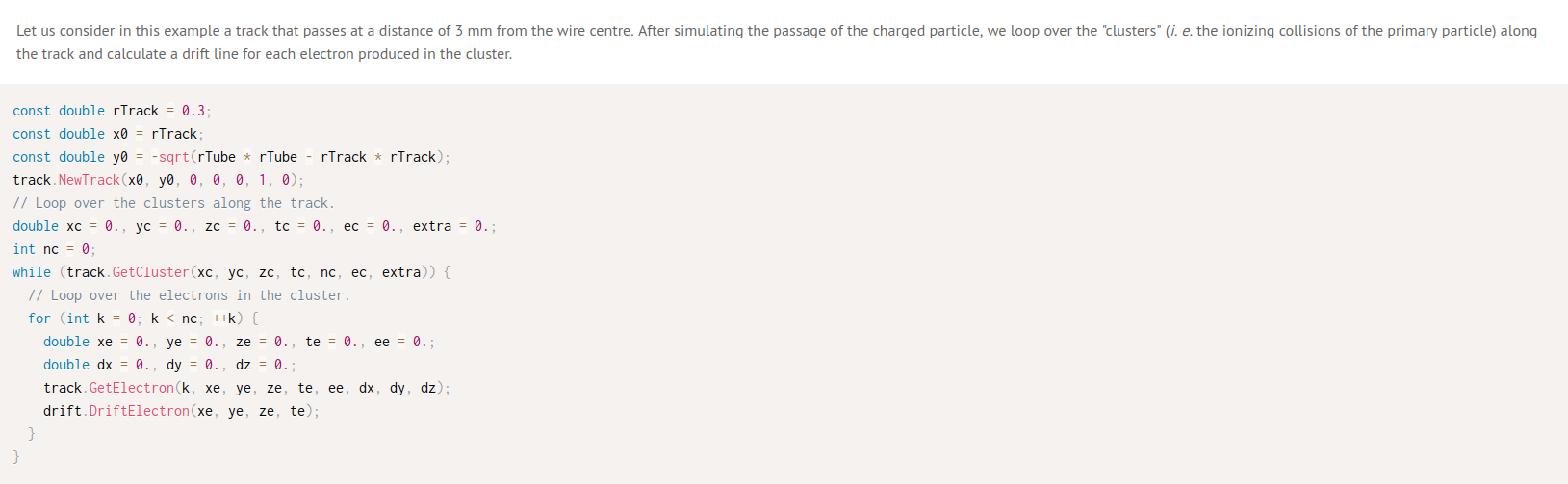
I want to get the drift line of the electron and proton, but the result shows that " Could not determine the plot limits." should I set the range of the particle trace in the beginning ? I just want the proton can pass through the whole gas area. I find a example in the drift tube, it define the particle passes at a distance of 3 mm from the wire centre. Dose that mean I should set the range of the trace?
Instead of a screen (very difficult to read) can you post a small macro reproducing your problem ? We can then execute it locally and fix it to make it work.
Indeed, a minimal working example would be very helpful.
You do not need to set the range of the particle track, only its starting point, time, and direction.
You have to make sure though that the initial position is in an active medium (i. e. in the gas in your case).
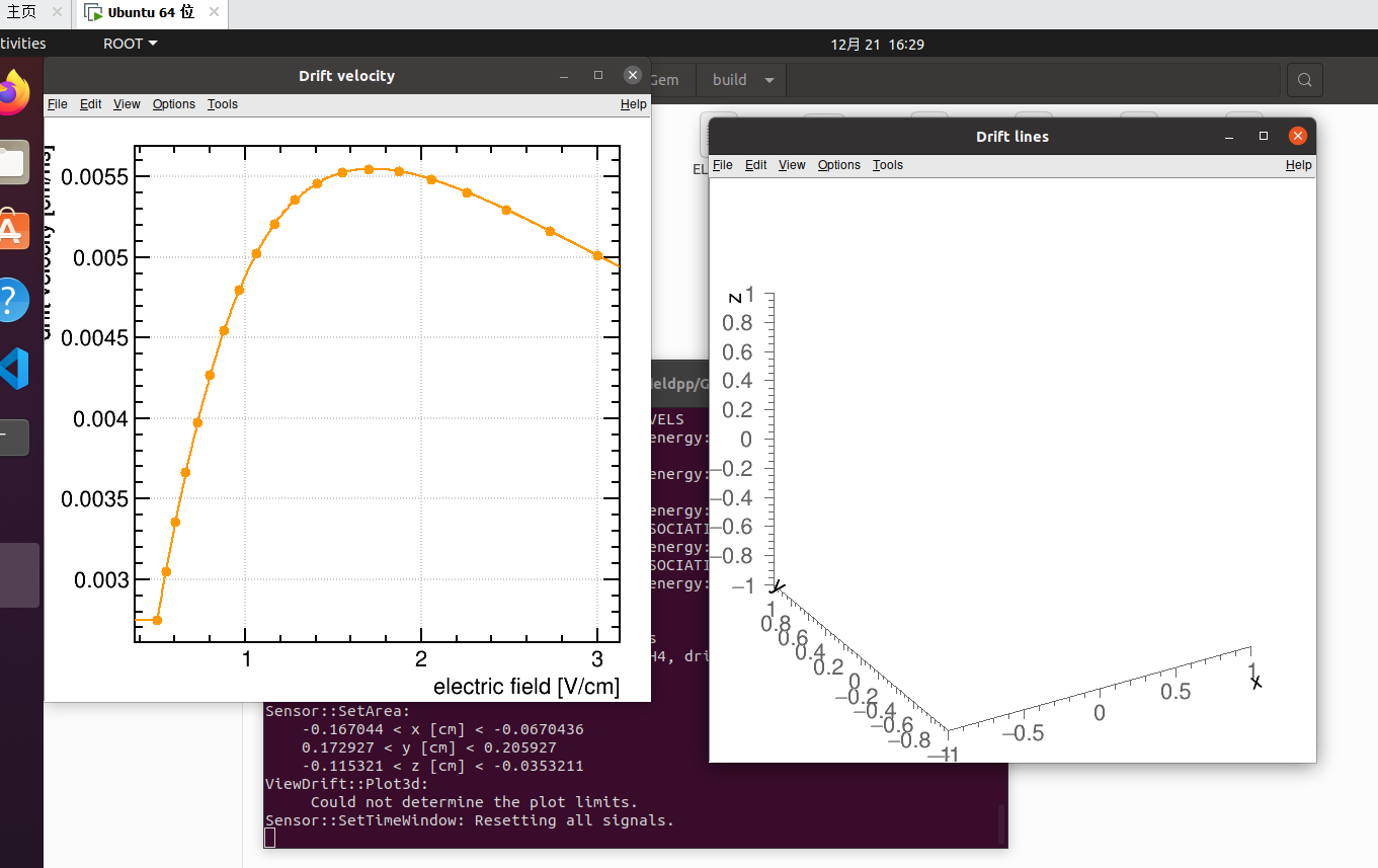
The message “Could not determine the plot limits.” comes from the class ViewDrift. If the plot limits are not set explicitly by the user (SetArea), ViewDrift will try to determine the plot range based on the extent of the drift lines to be plotted. I suspect that the reason you see this message is that there are no drift lines present.
Hi,
Thanks a lot for your reply
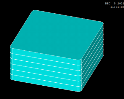
So would you please tell me what’s the reason for no drift lines, does that means something wrong with the model? I have set six gas air area,each of them has a slice gap, is the gap be the reason for the particle killed?
Hi,Thanks a lot for your reply
Sorry , I don’t know how to post a small macro reproducing my problem, my model is imported from the ansys, and I am the novice of Garfield++, So I don’t know how to show the problem.
Just post (a minimal version of the) source code of the macro/program you are running.
#include <iostream>
#include "Garfield/MediumMagboltz.hh"
#include "Garfield/FundamentalConstants.hh"
#include <cstdlib>
#include <fstream>
#include <TROOT.h>
#include <TApplication.h>
#include <TCanvas.h>
#include <TH1F.h>
#include <TTree.h>
#include <TFile.h>
#include "Garfield/ViewDrift.hh"
#include "Garfield/ComponentAnsys123.hh"
#include "Garfield/ViewField.hh"
#include "Garfield/ViewFEMesh.hh"
#include "Garfield/Sensor.hh"
#include "Garfield/AvalancheMicroscopic.hh"
#include "Garfield/AvalancheMC.hh"
#include "Garfield/Random.hh"
#include "Garfield/TrackHeed.hh"
#include "Garfield/DriftLineRKF.hh"
#include "Garfield/ViewMedium.hh"

using namespace Garfield;

int main(int argc, char * argv[]) {

  TApplication app("app", &argc, argv);
  //SetDefaultStyle();
// Load the field map.
  ComponentAnsys123 fm;
  fm.Initialise("ELIST.lis", "NLIST.lis", "MPLIST.lis", "PRNSOL.lis", "cm");
  fm.PrintRange();
  fm.PrintMaterials();
// Get the extent of the field map.
  double x0, y0, z0, x1, y1, z1;
  fm.GetBoundingBox(x0, y0, z0, x1, y1, z1);

  ViewField fieldView;
  constexpr bool plotField = true;
  if (plotField) {
    fieldView.SetComponent(&fm);
    // Set the normal vector of the viewing plane (xz plane).
    fieldView.SetPlane(0, 0, -1, 0, 0, 0.5 * (z0 + z1));
    fieldView.PlotContour();
    std::vector<double> xf;
    std::vector<double> yf;
    std::vector<double> zf;
    fieldView.PlotFieldLines(xf, yf, zf, true, true, kOrange-3);
  }

  Sensor sensor;
  sensor.AddComponent(&fm);//calculate the field

  // Setup the gas.
  MediumMagboltz gas;
  gas.LoadGasFile("4He.gas");
  gas.PrintGas();
  fm.SetMedium(0, &gas);
  fm.PrintMaterials();

  ViewMedium view;
  view.SetMedium(&gas);
  view.PlotElectronVelocity('e');

  // Track class
  TrackHeed track;
  track.SetParticle("proton");
  track.SetEnergy(100.e9);
  track.SetSensor(&sensor);

   //RKF integration
  DriftLineRKF drift;
  drift.SetSensor(&sensor); //chuanganqidaoru
  drift.EnableSignalCalculation();

  ViewDrift driftview;
  //the visualize of the electron drift
  TCanvas* CD= nullptr;
  constexpr bool plotDrift = true;
  if (plotDrift)
  {
    CD = new TCanvas("CD", "", 600, 600);
    const bool twod = false;
  	const bool axis = true;
    driftview.SetCanvas(CD);
    driftview.Plot(twod,axis);
    drift.EnablePlotting(&driftview);//plot the track of electron
    track.EnablePlotting(&driftview);//plot the track of proton
  }

  //the calculation of the transportation
  const unsigned int nTracks = 1;//one proton
  double counts,counts_e=0;
  for (unsigned int j=0; j < nTracks; ++j)
  {
    sensor.ClearSignal();
    double x0 = -0.1, y0 = 0.204, z0 = -0.07, t0 = 0.;  //make sure the start point of the proton and the direction
    double dx0 = 0., dy0 = 1., dz0 = 0.;
    track.NewTrack(x0, y0, z0, t0, dx0, dy0, dz0);
    double xc = 0., yc = 0., zc = 0., tc = 0., ec = 0., extra = 0.;
    int nc=0;

    //loop clusters
    while (track.GetCluster(xc, yc, zc, tc, nc, ec, extra))//loop clusters,gain the information of each cluster
    {
      counts++;
      cout<<"cluster position: "<< xc <<"\t"<< yc <<"\t"<< zc<<endl;

      //loop electrons in a cluster
      for (int k = 0; k < nc; k++)//loop electrons in a cluster,one cluster has nc number of electrons
      {
        double xe = 0., ye = 0., ze = 0., te = 0., ee = 0.;
        double dx = 0., dy = 0., dz = 0.;
        track.GetElectron(k, xe, ye, ze, te, ee, dx, dy, dz);//gain the electron information in one cluster
        drift.DriftElectron(xe, ye, ze, te);//calculate the drift of the electron

      }
    }

  }
  app.Run(true);
}
Hi,
Thanks a lot for helping me . I have post the source code of the program I am running
Thanks. You need to call driftview.Plot(twod,axis); after simulating the charged particle track and electron drift lines. If you call it before there are not drift lines present to be plotted.

Looks like the process was killed by the kernel (maybe because it ran out of memory).
I can’t say offhand what’s the reason for that, but I noticed something else when reading your code. The starting point is at the “top edge” of the geometry and the direction vector is (0, 1, 0). I guess you meant to use (0, -1, 0) instead, otherwise the proton has a high chance of escaping from the detector before it ionises.
I would also start with simulating and visualising a single electron drift line, and once you have checked that this works fine move on to simulating a charged particle track.
Hi,
Thanks a lot for your reply.
you are so meticulous,yes the direction vector actually should be -1. I have modified it ,and start with simulating and visualising a single electron drift line by setting the K value from K<nc to K<1. But the result seems the same, after get the bounding box, then killed.
 //loop electrons in a cluster
      for (int k = 0; **k < 1**; k++)//loop electrons in a cluster,one cluster has nc number of electrons
      {
        double xe = 0., ye = 0., ze = 0., te = 0., ee = 0.;
        double dx = 0., dy = 0., dz = 0.;
        track.GetElectron(k, xe, ye, ze, te, ee, dx, dy, dz);//gain the electron information in one cluster
        drift.DriftElectron(xe, ye, ze, te);//calculate the drift of the electron
      }
Hi,
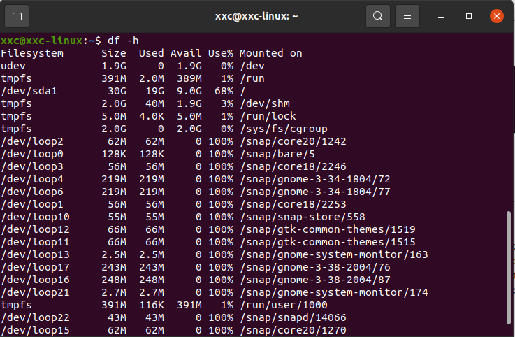
That’s the running results in the below
xxc@xxc-linux:~/garfieldpp/Gem/build$ ./gem
ComponentAnsys123::Initialise:
Read properties of 2 materials from file MPLIST.lis.
ComponentAnsys123::Initialise:
Read 2159067 elements from file ELIST.lis,
highest node number: 3124105,
background elements skipped: 0
ComponentAnsys123::Initialise:
Read 3124105 nodes from file NLIST.lis.
ComponentAnsys123::Initialise:
Read 3124105 potentials from file PRNSOL.lis.
ComponentAnsys123::Prepare:
Caching the bounding boxes of all elements... done.
ComponentAnsys123::InitializeTetrahedralTree: Success.
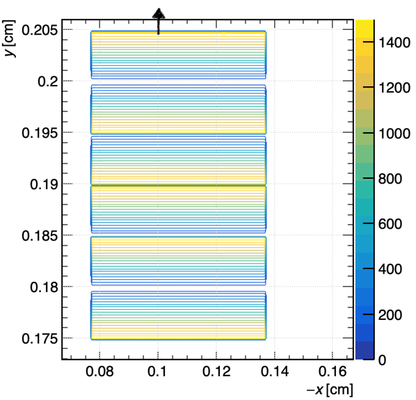
ComponentAnsys123::PrintRange:
Dimensions of the elementary block
-0.167044 < x < -0.0670436 cm,
0.172927 < y < 0.205927 cm,
-0.115321 < z < -0.0353211 cm,
0 < V < 1500 V.
Periodicities
x: none
y: none
z: none
ComponentAnsys123::PrintMaterials:
Currently 2 materials are defined.
Index Permittivity Resistivity Notes
0 1 -1 (drift medium)
1 4.25 1e+10
MediumMagboltz::LoadGasFile:
Reading file N2.gas.
Version 12.
Gas composition set to N2.
MediumMagboltz::PrintGas:
Gas composition: N2
Pressure: 10 Torr
Temperature: 293.15 K
Gas file:
Pressure: 10 Torr
Temperature: 293.15 K
Electric field range: 0.5 - 3 V/cm in 19 steps.
Magnetic field: 0 T
Angle between E and B: 1.5708 rad
Available electron transport data:
Velocity along E
Velocity along Bt
Velocity along ExB
Low field extrapolation: constant
High field extrapolation: linear
Interpolation order: 2
Longitudinal diffusion coefficient
Transverse diffusion coefficient
Diffusion tensor
Low field extrapolation: constant
High field extrapolation: linear
Interpolation order: 2
Townsend coefficient
Low field extrapolation: constant
High field extrapolation: linear
Interpolation order: 2
Attachment coefficient
Low field extrapolation: constant
High field extrapolation: linear
Interpolation order: 2
Lorentz Angle
Low field extrapolation: constant
High field extrapolation: linear
Interpolation order: 2
Ionisation rates
N2 IONISATION N2+ X2SIGMA VIB=0 ELOSS= 15.581
Threshold = 15.5807 eV
N2 IONISATION N2+ X2SIGMA VIB>0 ELOSS= 15.855
Threshold = 15.8547 eV
N2 IONISATION N2+ A2PI VIB=0 ELOSS= 16.699
Threshold = 16.6987 eV
N2 IONISATION N2+ A2PI VIB=1 ELOSS= 16.935
Threshold = 16.9347 eV
N2 IONISATION N2+ A2PI VIB>1 ELOSS= 17.171
Threshold = 17.1707 eV
N2 IONISATION N2+ B2SIGMA ELOSS= 18.751
Threshold = 18.7506 eV
N2 IONISATION N2+ C2SIGMA ELOSS= 23.591
Threshold = 23.5905 eV
N2 DISSOC ION (N+,N) ELOSS= 24.294
Threshold = 24.2935 eV
N2 DISSOC ION (N+,N*) ELOSS= 24.4
Threshold = 24.3995 eV
N2 DISSOC ION (N+*,N) ELOSS= 35.7
Threshold = 35.6993 eV
N2 DISSOC ION (N++,N) AND (N+,N+) ELOSS= 38.8
Threshold = 38.7992 eV
N2 IONISATION K-SHELL ELOSS= 401.6
Threshold = 401.592 eV
Low field extrapolation: constant
High field extrapolation: linear
Interpolation order: 2
Available ion transport data:
none
Killed
Hi,
Thanks for your advice, I will try to execute “ulimit -s unlimited” BEFORE I start my executable to see whether it can fix.
Hi,
the reason you don’t see any drift lines is that the proton has very little chance to ionize the gas before it leaves the detector.
I don’t have your gas file, so I used another one (the one from the drift tube example) to run (a slightly modified version of) your program. In my version of the program (which you’l find attached) I added a line track.Initialise(&gas, true); to print out some information about the ionisation cross-section of the charged particle. For the gas file I’m using, which is at a pressure of 3 atmospheres, the cluster density (average number of ionising collisions per track length) is about 100 / cm.
Your field map has a length of 300 um along y. So, with the gas file I’m using, the charged particle should on average have about 3 ionising collisions (=clusters) inside the detector. I’ve run the program a few times and this seems about right, that is I did get a couple of clusters and electron drift lines.
The gas file you are using is for a pressure of 10 Torr though, so the cluster density is very low and that’s why in most cases there will be no clusters, and thus no drift lines in your plot.
test.C (2.7 KB)
Hi,
Thanks for your help.
I don’t know how to say, you are indeed a Garfield++ master, what you say is clear and intelligible.
I have modified the pressure to 750 Torr which is the biggest pressure of the detector, maybe the detector’s design approaches to the vacuum condition.
Thanks again!