How does the lite Beeston-Barlow method implemented in HistFactory work?

[correian]

Hello everyone,

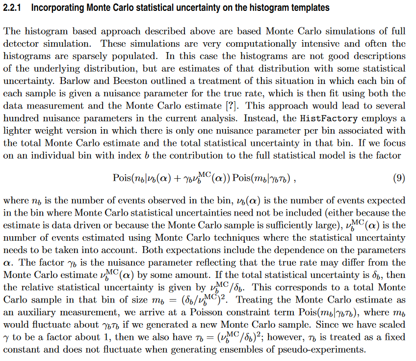
I have been trying to understand the lite version of the Beeston-Barlow method, that allows to take into account the limited statistics of the MC samples the fit templates are built from directly during the fit. This method is explained with precision in the following preprint article, in section 2.2.1 (an image is attached below). However, I’m still struggling to understand some piece of notation that were used, even though some of them were partially answered in this topic that dates back to 2018.

In the lite method, instead of varying the bin counts of each sample, this is done globally for all the MC samples. This means only one bin-wise scale factor gamma_b per bin b is defined, and is somehow constrained to vary under the overall MC statistical uncertainty.
Here are a list of questions I unfortunately can’t get past

1. sigma_b is defined as the total statistical uncertainty. Is it the total statistical uncertainty of the MC samples stacked together? So is it just sqrt(uncertainty_bin_b_sample_1^2 + uncertainty_bin_b_sample_2^2 + ...), where uncertainty_bin_b_sample_1 is either

• sqrt(counts in bin b for the sample 1) for an unweighted sample,
• sqrt(sum of squared weights for events belonging the sample 1 and bin b) for a weighted sample

Is that right? Or does the computation of sigma_b also involves the yields of their templates in the fit?

2. nu_b^MC is, from my understanding, just the amount of observed events in the bin b that are modeled by MC samples, so this is just sum over the samples s [(counts in bin b in sample s) / (total number of events in the sample s) * yield of the component s found by the fit].

3. tau_b (which, I guess, is supposed to represent the “statistical power” of the MC samples in the bin b) is computed as (vu_b^MC / delta_b)^2, and is “treated as a fixed constant and does not fluctuate when generating ensembles of pseudoexperiments”. Does this mean that tau_b^MC does not change during the fit, so nu_b^MC is computed at the start of the fit according the starting point of the fit, and is then unchanged during the fit?

4. Finally, despite the explanations in the 2018 topic, I do not understand why gamma tau_b = gamma (nu_b^MC/delta_b)^2 is the quantity that is constrained, and that it is the size of total monte carlo sample in that bin. nu_b^MC and delta_b seem to be unrelated quantites, as nu_b^MC, on the one hand, is predicted by the fit, and is solely related to the data that is being fitted. On the other hand, delta_b seems to be only related to the MC statistics.

I’m sorry for such a long message, with so many questions, and if don’t understand something that is completely obvious or annoying to explain, or if my message is confusing.

Thanks for any answers,
Anthony.

PS: I’ve been trying to understand how this method works in order to use it together with the python library zfit. I know that another python library, pyhf, closely related to HistFactory, has implemented the lite Beeston-Barlow method, but with Gaussian constraint. The way to do it with Poisson constraint using their framework is still unclear to me.

…

"Normal" Beeston-Barlow method

The “normal” Beeston-Barlow method seems clear to me, it is very well explained in the original 1993 paper. In brief, the number of generated candidates for each bin of each MC sample is Poisson-constrained, instead of just being a constant. This way, if the MC sample does not contain enough statistics to represent well enough the true underlying PDF (Probability Density Function), the bin counts for each sample can slighly accomodate. Then you can either minimise the overall likelihood or equivalently solve some equations iteratively).

In, this paper, the factor needed to normalise the histogram and scale the template are explicitely given in equation (1). The parameters of the constrained terms look also easier to compute and understand because you do not need to combine the statistical uncertainty of different MC samples that can appear with different (possibly varying) yields in the fit.

[jonas]

Hi @correian thanks for your detailed questions!

1. Yes that’s completely correct what you describe. It’s the squared-sum of uncertainty histograms that the user passes to HistFactory for the samples. You can see how it is implemented in HistoToWorkspaceFactoryFast::MakeScaledUncertaintyHist().
2. nu_b^MC is calculated even more direct than you write, as the histograms used to create samples in HistFactory are directly the pre-fit yields. So if there are no other parameters alpha that scale/morph the histogram shapes, it doesn’t even depend on the data and is just sum over the samples s [histogram content for sample s].
3. That’s also correct! Tau is constant, computed just from the uncertainties obtained like I said in bullet point 1: tau_b = 1/relative_delta_^2. You can find this here in the code.
4. Right, nu_b^MC(alpha) and delta_b are unrelated if you want to call it like that. nu_b^MC(alpha) are found by the fit (or constant if there are no other parameters alpha), while delta_b is used to constrain gamma.

I think what probably caused the confusion is that in the text you inserted to your post, nu_b^MC and nu_b^MC(alpha) are not the same. The nu_b^MC is the initial shape for a sample, and nu_b^MC(alpha) is changing with the fit.

Hope that clarifies things a bit, let me know if I should follow up on something!

Cheers,
Jonas

[correian]

Hello @jonas,
Thanks a lot for this answer and for the links to the source code! The method appears crystal clear to me now! Thanks to your explanations, I’ve been able to use it with zfit in a small toy example.
Indeed, you are right, I thought nu_b^MC and nu_b^MC(alpha) were the same!

Cheers,
Anthony.