Hard constraints for implicit parameters

[JanEric]

Hi,

we are reparametrizing a HistFactory model from signal strengths to fractions.

(mu_1, mu_2, mu_3) → (f_1, f_2, mu_tot)

And f_3 is implicitly defined as (1-f_1-f_2)

However, this parametrization has the problem that the physical boundaries can not be guaranteed for the implicit f_3 fraction.

For the mu parameters hard boundaries can be set, for example a lower one of 0.
The same can be done for the explicit fractions alongside a hard upper bound of 1.

With this all fractions sum to one and all are guaranteed to be <= 1.
However, the f_3 fraction can become negative as both f_1 and f_2 can in principle become 0.8 for example.

Is there anyway to apply a hard boundary on implicit parameters like f_3 as it is possible with the explicit ones like mu_1 or f_1?

I have tried using external constraints for the fit with something like

RooFormulaVar x(..., ..., "1-f1-f2", RooArgSet(f1, f2))
RooGenericPdf constraintPdf(..., ..., "(x<0)*x*x*x*x + (x>1)*x*x*x*x", x);

but that always either still yielded unphysical values for f_3 or made the fit unstable.
So I am wondering how the hard cuts work for the explicit parameters and if it is possible to apply the same approach for the implicit ones?

Cheers
Jan-Eric

[Ako_b]

Hello, @JanEric !
A possible solution could be to use following parametrization:

f_1 = u

f_2 = v (1 - u)

f_3 = 1 - u - v (1 - u)

where 0 \leq u, v \leq 1.
It is based on the fact that f_2 \leq 1 - f_1, then just rescaling f_2

Another parametrization is based on spherical coordinates.

f_1 = \sin^2 \theta \cos^2 \phi

f_2 = \sin^2 \theta \sin^2 \phi

f_3 = \cos^2 \theta

f_1 + f_2 + f_3 = 1

However, as this is non-linear transformation, it can affect fit stability and introduce local extrema.

[JanEric]

The simplest parametrization would probably just be the normal signal strengths.

We wanted to try to explicitly use the one given above as that is the physics target and would allow us to directly use the (asymmetric) uncertainties without any after-the-fact propagation.

We also have another (physics motivated) parametrization which suffers from this problem even worse. I guess there is not easy way to introduce HARD constraints like the ones present on explicit fit parameters?

[Ako_b]

Could you please provide minimal working example?
I didn’t encounter any difficulties with test macro below. It seems that RooFit can handle such a use case automatically.

// fit.cpp
void fit() {
    RooRealVar x("x", "x", -10, 10);
    RooRealVar mean1("mean1", "mean1", 0, -10, 10);
    RooRealVar mean2("mean2", "mean2", 1, -10, 10);
    RooRealVar mean3("mean3", "mean3", 2, -10, 10);
    RooRealVar sigma1("sigma1", "sigma1", 0.5, 0.1, 10);
    RooRealVar sigma2("sigma2", "sigma2", 0.25, 0.1, 10);
    RooRealVar sigma3("sigma3", "sigma3", 0.1, 0.1, 10);

    RooGaussian g1("g1", "g1", x, mean1, sigma1);
    RooGaussian g2("g2", "g2", x, mean2, sigma2);
    RooGaussian g3("g3", "g3", x, mean3, sigma3);

    RooRealVar f1("f1", "fraction of component 1 in signal", 0.5, 0., 1.);
    RooRealVar f2("f2", "fraction of component 2 in signal", 0.3, 0., 1.);
    RooRealVar nsig("nsig", "number of signal events", 10000, 0., 1000000);

    // value of f3 = 1 - f1 - f2 is inferred automatically
    RooAddPdf sig("sig", "f1 * g1 + f2 * g2 + f3 * g3", RooArgList(g1, g2, g3), RooArgList(f1, f2));

    RooExtendPdf model("model", "extended signal pdf", sig, nsig);

    int nevents = 100000;
    std::unique_ptr<RooDataSet> data{model.generate(x, nevents)};

    model.fitTo(*data, RooFit::PrintLevel(-1));

    RooPlot *xframe = x.frame(RooFit::Title(""));

    data->plotOn(xframe);
    model.plotOn(xframe, RooFit::Normalization(1.0, RooAbsReal::RelativeExpected));
    model.Print("t");

    new TCanvas("canvas", "", 600, 600);
    gPad->SetLeftMargin(0.15);
    xframe->GetYaxis()->SetTitleOffset(1.4);
    xframe->Draw();
}

[JanEric]

Wow, i didnt know that this works without specifying the 1-f1-f2.

What i am doing is following this approach here (slide 46): https://indico.cern.ch/event/634161/contributions/2678994/attachments/1524553/2383382/armbruster.pdf
https://gitlab.cern.ch:8443/armbrust/RooFit-tutorial/-/blob/master/macros/parametrizeShape.C

And with that i am seeing cases where all of the set fraction reach values like 0.8, leading to the 1-f1-f2 term to become negative. I can try to adjust one of the example to make the issue occur.

But we also have a more complicated parametrization where an implicit sum would not solve the issue.
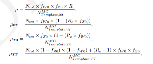
Here are the parametrization i have used. The \mu are normalization factors in histfactory as added by sample.AddNormFactor(*settings). And the f’s refer to the parts of the formulas without the N_{tot} and N_{Tempalte}

[Ako_b]

@JanEric

https://gitlab.cern.ch:8443/armbrust/RooFit-tutorial/-/blob/master/macros/parametrizeShape.C

Unfortunately, I can’t access this file.

@JanEric

But we also have a more complicated parametrization where an implicit sum would not solve the issue.
Here are the parametrization i have used.

I can’t say much about this because I don’t have enough context, understanding which may require some specialized knowledge beyond my experience.
So I can make only a heuristic guess.
If we rewrite the parametrization a little

\mu_{} \frac{N_{\text{Template},00}^{\text{MC}}}{N_\text{tot}} = f_{W0} f_{Z0} - (1 - R_c) f_{W0} f_{Z0}

\mu_{0T} \frac{N_{\text{Template},0T}^{\text{MC}}}{N_\text{tot}} = f_{W0} (1 - f_{Z0}) + (1 - R_c) f_{W0} f_{Z0}

\mu_{T0} \frac{N_{\text{Template},T0}^{\text{MC}}}{N_\text{tot}} = (1 - f_{W0}) f_{Z0} + (1 - R_c) f_{W0} f_{Z0}

\mu_{TT} \frac{N_{\text{Template},TT}^{\text{MC}}}{N_\text{tot}} = (1 - f_{W0}) (1 - f_{Z0}) - (1 - R_c) f_{W0} f_{Z0}

then, assuming that 0 \leq f_{W0}, f_{Z0} \leq 1, I would say that the factor (1 - R_c) should be a correction to some base model which treats W0 and Z0 as independent variables.
Hence, my intuition is that it should be at least |1 - R_c| \leq 1, which is not the case for the data you’ve provided and that would explain out of bounds values of f fractions.
However, I must emphasize that it is just a guess.

[JanEric]

Unfortunately, I can’t access this file.

Ah, unfortunate, i am not sure if i am allowed to just copy paste the content.

Yeah. You are pretty spot on with what the parametrization represents. We have two particles (W and Z) which can either be in a (polarization) state of “0” or “T”. The standard way to represent this is to have four fractions f_{00},f_{0T},f_{T0},f_{TT}. Where one is eliminated to make them sum to one.(And in a fit we also use another parameter to scale all of them together).

But we now want to not investigate the individual fraction but whether they are compatible with the states of the two particles being independent.

If they are independent then we expect f_{00}=f_{W0} \times f_{Z0}. So above that would be equivalent to R_c=1. If they are not, then R_c can take any value between 0 and infinity. (depending on f_{W0} and f_{Z0}. The issue is that we can not constrain f_{T0} and f_{0T} well in data. Only their sum. And this then results in values like

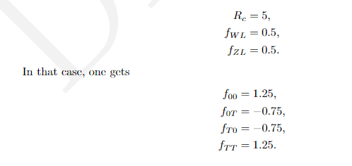
R_c = 10, f_{W0}=0.04, f_{Z0} = 0.49. And if you plug that into the above formulas you get negative values for f/\mu_{0T}. And i would need a way to constrain the combinations of R_c, f_{W0}, f_{Z0} to physical regions. I tried adding constraint terms that that the forumale f_{W0} \times (1-( R_{c} \times f_{Z0} gets penalized if it is below 0 or above 1 times the same things for all the others. But that makes the fit extremely unstable and constraints are also not hard. If that region is otherwise favoured then it still goes into the unphysical region, just less deep.