Generating correlated random numbers using correlated matrix from MINUIT

[amroo]

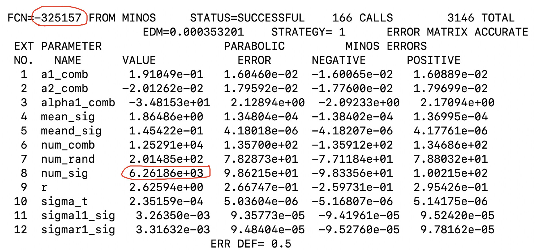
Fit1> signal dataset, obtain a pdf using MIGRAD followed by MINOS

Fit2> background dataset, obtain a pdf using MIGRAD followed by MINOS

Fit3> Signal + background dataset, use the pdf obtained in Fit1 and Fit2, fixing some shape parameters
from the results of Fit1 and Fit2, floating other parameters.

Now I want to evaluate the systematic uncertainty to final signal yield from fit3 due to the fixed shape parameters.
say the value is afi±del_afi for parameter i,

To evaluate the systematic uncertainty,
I am performing 5000 fits of my data set. For each fit cycle, the value of fixed-parameters is sampled from a gaussian pdf with mean afi and sigma delta_afi

I have 31 such fixed parameters, and many of them are correlated (known from the correlation matrix of fit1 and fit2).

Is there a way in roofit to include the correlation between these shape parameters randomly sampled values for each such fit cycle?

[bellenot]

@moneta will most probably help you with this

[Eddy_Offermann]

I am not familiar enough with roofit to know if a method exists in this package, but it would take just a handful of lines using TMatrixD following this example:
https://scipy-cookbook.readthedocs.io/items/CorrelatedRandomSamples.html

[moneta]

Hi,
You can do in RooFit, creating a multi-dimensional Gaussian pdf and generate events from that distribution. But I think, since you need just the parameter values that you will use for your fits, you can follow the procedure shown by Eddy.
We have also an open PR for adding this in ROOT, based on GSL. See Add multivariate random number generation by jolopezl · Pull Request #7186 · root-project/root · GitHub, I think we will add this new contribution soon in ROOT master

Best regards

Lorenzo

[moneta]

Hi,
The code to generate multi-dimensional gaussian random numbers is now available in ROOT, see the tutorial root/multivarGaus.C at master · root-project/root · GitHub

Lorenzo

[amroo]

Hi @moneta , Thanks for a very quick response

I get the error " no member named ‘GaussianND’ in ‘ROOT::Math::GSLRandomEngine’ while trying to implement the code :root/multivarGaus.C at master · root-project/root · GitHub

My macro is attached:
test_random1.C (2.2 KB)
sigf_SM.root (12.9 KB)

I am using root version: 6.22/08

[amroo]

Thanks for your reply @Eddy_Offermann

Along with the process suggested by moneta. I also want to try the method suggested by you:

To do that
I have a TMatrixD randx(12,1); matrix filled with uncorrelated random numbers sampled from Gaussian distributions
The covariance matrix is : TMatrixDSym cov_l1m(12,12);

To apply the Cholesky decomposition I am doing
TDecompChol rd(cov_l1m);

then generate a matrix of correlated random numbers y as
TMatrixD randy = rd*randx;

But this last line doesn’t compile, Can you point out the problem here?
See the attached macro:
test_random.C (2.0 KB)
sigf_SM.root (12.9 KB)

Thanks

[moneta]

Hi,

You cannot use version 6.22 for this, but the ROOT master version, 6.25. You would need to build it from source, cloning the HEAD of the ROOT github repository,

root-project/root

Lorenzo

[Eddy_Offermann]

Use

TMatrixD randy = rd.getU()*randx;

[amroo]

@moneta

You cannot use version 6.22 for this, but the ROOT master version, 6.25. You would need to build it from source, cloning the HEAD of the ROOT github repository,

Ok it works. But there is still one problem

Changing from Root 6.22 → 6.25 ,
RooFit results from same macro and dataset changes

Result from Root 6.22:

Result from Root 6.25:

num_sig: circled in the figures is significantly different between the two results

[amroo]

@Eddy_Offermann
I am having problem filling the matrix:
I am following Chapter: LinearAlgebra

Below is the code I am using to fill matrix:

 TArrayD cov_l1(144);
   TMatrixDSym cov_l1m(12,12); //matrix to store the reduced covariance matrix                                                                         
   int fill_indx=0;
   for(int i=0;i<12;i++)
     {
       for(int j=0;j<12;j++)
         {                                                                                           
           cov_l1[fill_indx] = cov(sel_indx[i],sel_indx[j]);         // cov is a TMatrixDSym matrix                                                                                                                                                                                                                          
           fill_indx++;
         }
     }
   cov_l1m.SetMatrixArray(cov_l1.GetArray());
   cout<<cov_l1m.GetNcols()<<endl;
   cout<<cov_l1m.GetNrows()<<endl;

But the last two cout commands only give me 1 as no. of rows and columns
I expect 12 ? I couldn’t figure out the mistake here

[Eddy_Offermann]

the TMatrixDSym constructor is here. So try

TMatrixDSym co_l1m(12);

Looking at your code you can skip the filling of the array and then filling the matrix by directly stating:

cov_l1m(i,j) = cov(sel_indx[i],sel_indx[j]);

[amroo]

@Eddy_Offermann
Thanks, I got everything working now. But the final results don’t make sense.
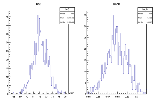
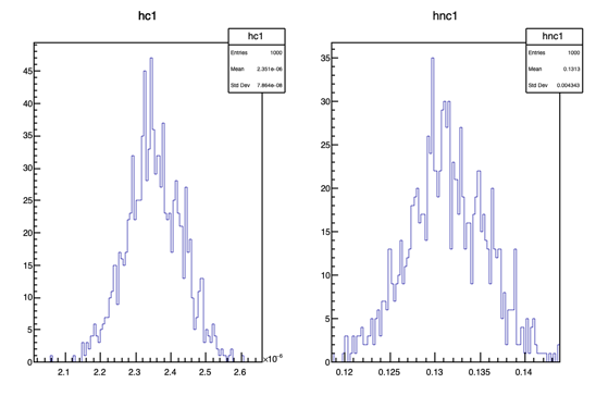
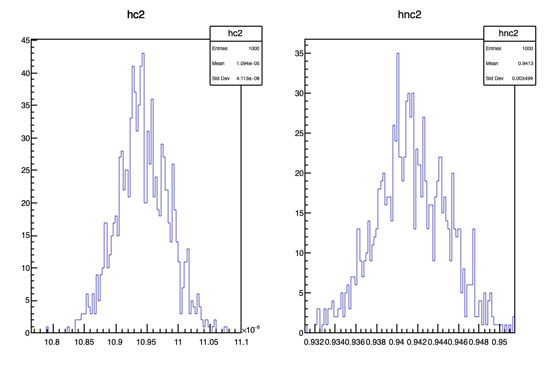
To test it. I have used a covariance matrix with off-diagonal elements as zero.
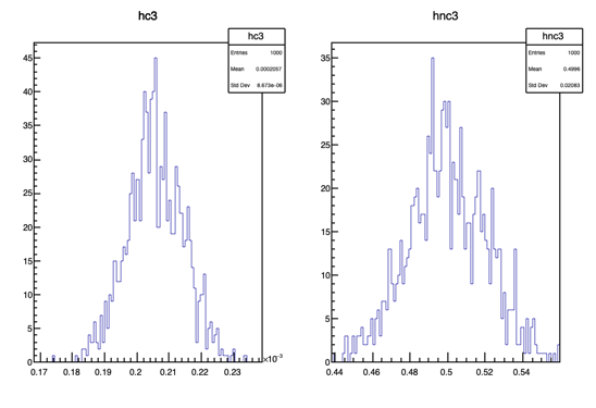
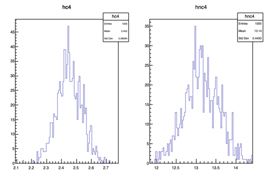
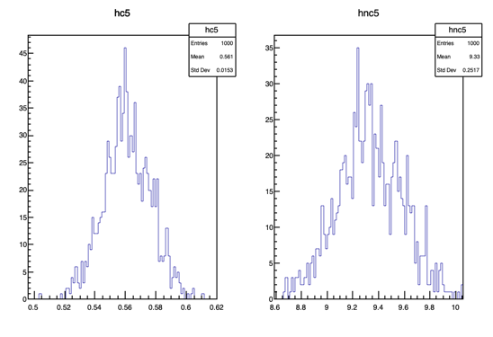
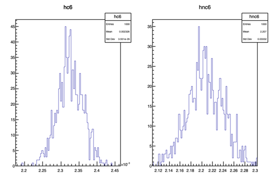
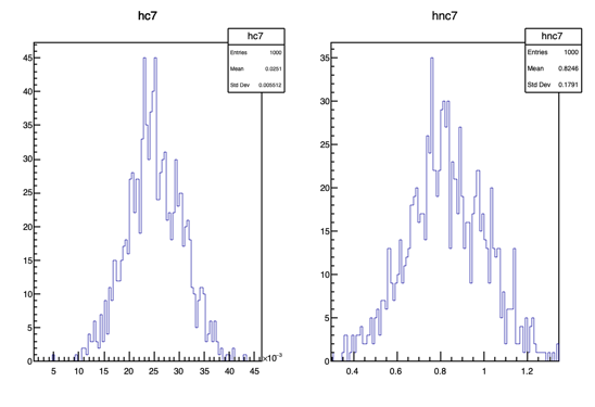
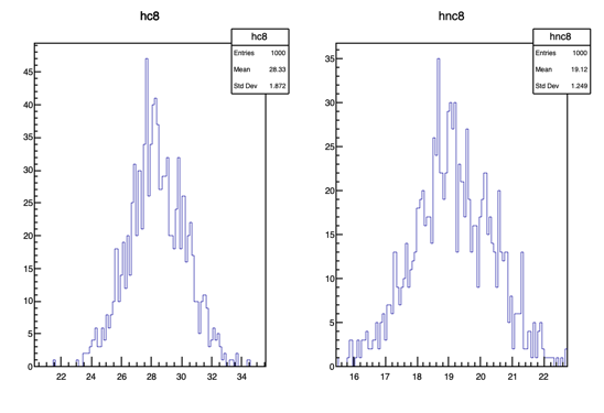
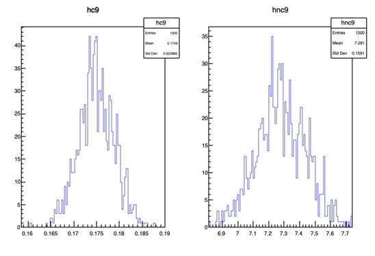
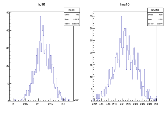
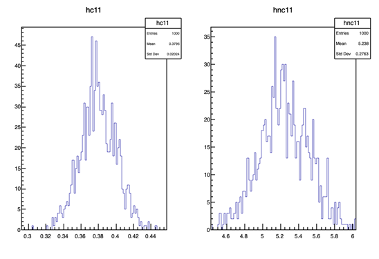
Compared the distributions of uncorrelated and correlated random variables from 1000 generation cycles.
They are expected to be the same given the covariance matrix is diagonal.
Covariance matrix used:

See the distributions below for 12 random variables. The distribution of correlated random variable is on left and the uncorrelated random variable is on right. Do you know what is going on here ?:
Also attaching my macro:
sigf_SM.root (12.9 KB)
test_random_diag.C (2.9 KB)

Also attaching plots in pdf format if plot below are not clear

canvas_cor_uncor0.pdf (16.1 KB)
canvas_cor_uncor1.pdf (16.0 KB)
canvas_cor_uncor2.pdf (16.1 KB)
canvas_cor_uncor3.pdf (16.0 KB)
canvas_cor_uncor4.pdf (15.8 KB)
canvas_cor_uncor5.pdf (15.8 KB)
canvas_cor_uncor6.pdf (16.0 KB)
canvas_cor_uncor7.pdf (16.0 KB)
canvas_cor_uncor8.pdf (15.9 KB)
canvas_cor_uncor9.pdf (15.9 KB)
canvas_cor_uncor10.pdf (15.8 KB)
canvas_cor_uncor11.pdf (15.9 KB)

[Eddy_Offermann]

That is what is expected if the matrix is not the identity, otherwise it is scaled by the qsrt of the diagonal.

[amroo]

Ok, so Instead of covariance matrix if I use a correlation matrix with off diagonal elements as zero. Then I should get same distributions. Just checked and the results are as expected same distributions.

But even with a covariance matrix with non-zero off diagonal elements, the two distributions should be identical. The only difference is if I plot a 2d distribution of x1 vs x2 , then it would be different from a non correlated case ?

May be I am really missing important conceptual point here? I am confused

Thanks

[Eddy_Offermann]

If you make the transformation on a gaussian distributed variable x

y = alpha * x

you will have a gaussian distributed variable y with a standard deviation

sigma(y) = alpha * sigma(x)

Here is a link to maybe an interesting course: coursera