Dear all,
I’m calculating a UL for a simple model sS+bB, where the S and B pdf is obtained from Histograms templates, for the UL calculation, I generate a pseudo data of 8 final events, which are only BKG events.
then for my model config, I do the following,
infile = ROOT.TFile.Open(input_factory)
w = infile.Get("w")
data = w.data("obsData")
#Model S+B
sbModel = w.obj("ModelConfig")
sbModel.SetName("S+B Model")
poi = sbModel.GetParametersOfInterest().first()
poi.setVal(0)
sbModel.SetSnapshot(ROOT.RooArgSet(poi))
#Model B
bModel = sbModel.Clone()
bModel.SetName(sbModel.GetName()+"_with_poi_0")
poi.setVal(0)
bModel.SetSnapshot(ROOT.RooArgSet(poi))

pc =ROOT.RooStats.ProofConfig(w, 0, " ", False)
fc = ROOT.RooStats.FrequentistCalculator(data, bModel, sbModel)
fc.SetToys(500,500)
calc = ROOT.RooStats.HypoTestInverter(fc)
calc.SetConfidenceLevel(0.90)
.... and so on
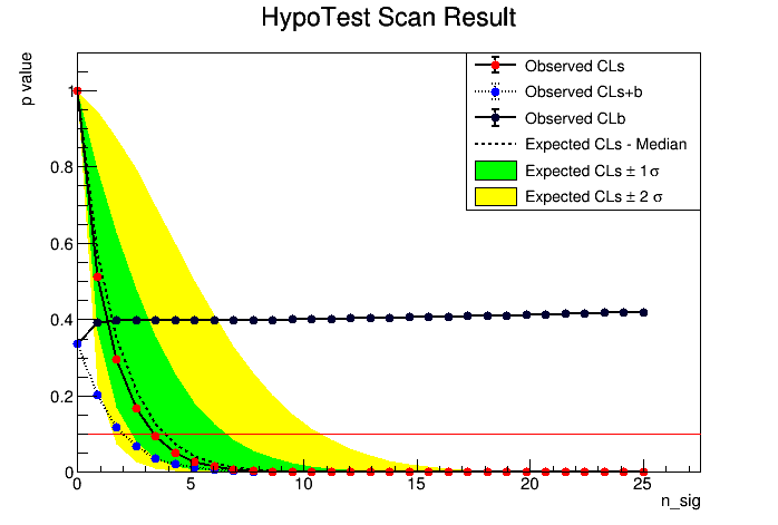
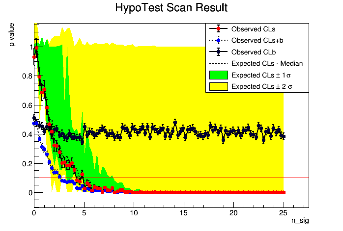
I calculated the UL using the asymptotic approximation and everything look ok (fig1_asym.png), however as this is a case of small statistics, I changed to the full frequentist implementation, however, the expected limit for 2sigmas is not converging for some reason (fig2_toys.png), in both cases, the model and pseudo data are the same only the calculator is changing, so why the expected UL for 2 sigmas is not calculated correctly for the full implementation case?.
I hope you can point me what are the differences in the expected UL calculation? I already change the scan range and the number of toys without any improvement.
On the other hand, if someone can tell me how can I print more information in the full implementation, for example, the final fit values. fig1_asym_ULresults.txt (328 Bytes) fig2_toys_ULresults.txt (316 Bytes)
Definitely, there is something wrong with the uncertainty bands of the FrequentistCalculator study, but it’s hard to tell what’s going on without more information. The difference between the UL computation with the asymptotic formulae and this toys is explained in section 5 of this reference. With the asymptotic formulae, the distribution of the test statistic is calculated analytically, using the value of the test statistic for the Asimov dataset. With toys, the test statistic distribution is determined by sampling from it.
But without seeing more of your fit, I can’t really give a good debug suggestion. Can you share as much information as possible? Optimally the full script with input files, or at least the full script and the output log. Have you tried increasing the verbosity levels so see if the profile likelihood fits converge?
Looking forward to follow up on this issue!
Cheers,
Jonas
Hi @jonas ,
Thanks for your response
I am attaching the wsfactory and the full script. Roostat_Freq.py (3.5 KB) 0Signal8Bkg_2Drot_12_ok.root (20.9 KB)
The yield have the limits s:[-20,25] and b: [-10, 80], and the SetFixedScan from [0,poi.getMax()=25].
I added to my script the SetPrintLevel(3) for the ProfileLikelihoodTestStat, I can see some warnings but I think at the end the fit converge, I don’t know If I can print more info, I’m very new using RooStats so I will really appreciate any help.
Thanks in advance.
PS.In the case of the asymptotic implementation, I checked the fits from 1000 pseudo data(toys), and under the same conditions, almost all looked ok.
sorry I was not able to debug the exact problem so far, it takes quite some time to debug this because the scrip takes some time to run each time.
What I have figured out so far is that the problem seems to be related to the fact that the nuisance parameter n_bkg is completely unconstrained in the model, which can also be seen when you print the workspace:
Maybe this is a problem in your model? I think the completely floating n_bkg in combination with the small event count in the experiment is the problem. I was thinking quite a bit about what effects this has, but I have no good intuition about this yet.
I think before discussing how to proceed further we should clarify: are you really sure that not constraining n_bkg at all is what you want to do in this fit? This would be very unusual. If you just forgot to add some constraints we can solve the problem easily: after adding some constraint to n_bkg like a Gaussian constraint around the background estimation of 8 events, the Brazilian plot looks fine.
Hi @jonas thanks for your reply, yes I wasn’t using any constrain as first test of this UL calculation, however, after the n_bkg constrain implementation in the model (I added the following lines)