Greetings,
an issue with the electron drift simulation in Garfield++ has been plaguing me for the past few days.
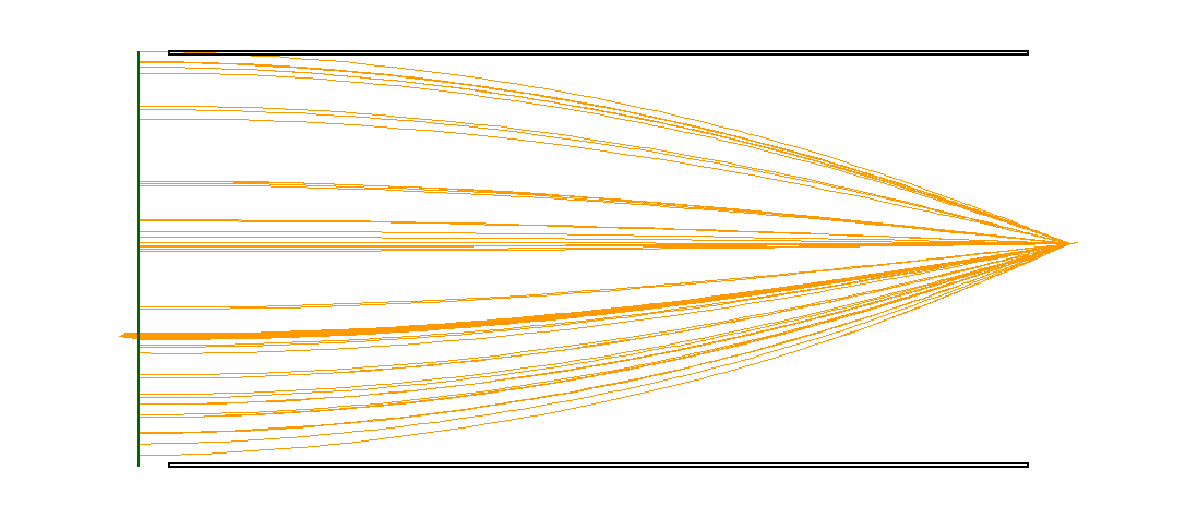
I have been trying to simulate the passage of a muon track inside a drift chamber cell that I had set up:
- I defined the structure of the cell using the native geometry (
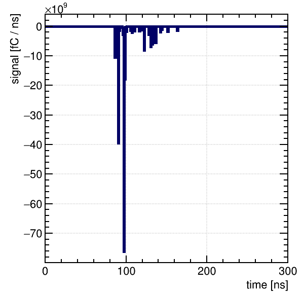
SolidBoxfor plates andSolidWirefor wires) and computed the electric field withComponentNeBem3d. - I then aimed at getting the signal induced on the central wire by a particle track, computing the drift lines with the
DriftLineRKFclass and plotting the induced signal and the simulated drift lines.
This is the code that I have been using:
#include <iostream>
#include <fstream>
#include <cstdlib>
#include <sys/stat.h>
#include <math.h>

#include <TCanvas.h>
#include <TROOT.h>
#include <TApplication.h>

#include "Garfield/ComponentNeBem3d.hh"
#include "Garfield/MediumMagboltz.hh"
#include "Garfield/MediumConductor.hh"
#include "Garfield/GeometrySimple.hh"
#include "Garfield/SolidBox.hh"
#include "Garfield/SolidWire.hh"
#include "Garfield/ViewGeometry.hh"
#include "Garfield/Sensor.hh"
#include "Garfield/DriftLineRKF.hh"
#include "Garfield/TrackHeed.hh"
#include "Garfield/ViewDrift.hh"
#include "Garfield/ViewSignal.hh"

using namespace Garfield;

int main(int argc, char * argv[]){

    TApplication app("app", &argc, argv);

    //load the gas medium for the internal space
    MediumMagboltz gas;
    gas.LoadGasFile("ar_85_co2_15_1atm.gas");
    //define the conductor material for the strips and wire
    MediumConductor plane_medium;
    MediumConductor strip_medium;
    MediumConductor wire_medium;

    //Defining the finite plane geometry through a GeometrySimple object
    GeometrySimple geo;

    //geometric parameters
    //----whole cell----
    //half-length of the assembly along z [cm]
    const double hlength = 100.;
    //gap half-length
    const double half_gap = 0.1;
    //half width of a cell
    const double cell_width = 1.;
    //half thickness of a cell
    const double cell_thick = 0.5*cell_width;

    //----strips----
    //half dimensions
    const double stripWidth = 1*cell_width-half_gap;
    const double stripThick = 35e-4;


    //----wires----
    //signal wire radius [cm]
    const double r_signal_wire=20.e-4/2;
    //field wire radius
    const double r_field_wire=100.e-4/2;

    //----Voltages----
    //strip voltage
    const double vStrip = -1000.;
    //signal wire voltage
    const double v_signal_wire = +1500.;
    //field wire voltage
    const double v_field_wire = -3500.;

    //define the cathode strips
    SolidBox c_strip_up(0.,cell_thick-stripThick,0.,stripWidth,stripThick,hlength);
    SolidBox c_strip_down(0.,-cell_thick+stripThick,0.,stripWidth,stripThick,hlength);
    //define the signal wire
    SolidWire sens_wire(0.,0.,0.,r_signal_wire,hlength);
    //set this wire as the electrode
    sens_wire.SetLabel("s");

    //define the field wires: left side
    SolidWire field_wire_u_l(-cell_width,0.,0.,r_field_wire,hlength);
    //define the field wires: right side
    SolidWire field_wire_u_r(+cell_width,0.,0.,r_field_wire,hlength);

    //set the boundary potentials for the components
    sens_wire.SetBoundaryPotential(v_signal_wire);
    field_wire_u_l.SetBoundaryPotential(v_field_wire);
    field_wire_u_r.SetBoundaryPotential(v_field_wire);
    c_strip_up.SetBoundaryPotential(vStrip);
    c_strip_down.SetBoundaryPotential(vStrip);

    //add wires strips and planes to the geometry
    geo.AddSolid(&sens_wire,&wire_medium);
    geo.AddSolid(&field_wire_u_l,&wire_medium);
    geo.AddSolid(&field_wire_u_r,&wire_medium);
    geo.AddSolid(&c_strip_up, &strip_medium);
    geo.AddSolid(&c_strip_down, &strip_medium);

    //add the boundary volume filled with gas
    geo.SetMedium(&gas);

    //Before moving on one needs to compute the field with neBEM
    ComponentNeBem3d nebem;
    nebem.SetGeometry(&geo);
    nebem.SetTargetElementSize(0.1);
    nebem.SetMinMaxNumberOfElements(20,20);
    nebem.SetNumberOfThreads(8);
    nebem.SetPeriodicityX(2*cell_width);
    nebem.Initialise();

    //Use a Sensor object to interface to the transport classes
    Sensor sensor;
    //add the field and electrode components
    sensor.AddComponent(&nebem);
    sensor.AddElectrode(&nebem,"s");

    const double tstep = 0.5;
    const double tmin = 0.;
    const unsigned int nbins = 100.;
    //setup the binning for the signal calculation (start, bin width[ns],bin number)
    sensor.SetTimeWindow(0.,1000.,nbins);
    sensor.SetArea(-cell_width,-cell_thick,-hlength,cell_width,cell_thick,hlength);

    //Simulating the ionization with Heed
    //first a track object is defined
    std::cout<<"-- Particle track simulation --"<<std::endl;
    TrackHeed track;
    track.SetParticle("muon");
    track.SetEnergy(170e9);
    track.SetSensor(&sensor);
    //compute the track
    track.EnableDebugging();

    //compute the electron drift lines
    DriftLineRKF drift;
    drift.SetSensor(&sensor);
    drift.UseWeightingPotential(false);
    drift.EnableAvalanche();
    drift.EnableSignalCalculation();

    //set the initial position: middle-left side of the cell
    const double x0 = -cell_width/2, y0 = -cell_thick, z0 = 0., t0 = 0.;
    //set the track direction and define the track
    const double dx0 = 0., dy0 = 1., dz0 = 0.;
    track.NewTrack(x0,y0,z0,t0,dx0,dy0,dz0);

    //loop over the clusters
    double xc = 0., yc = 0., zc = 0., tc = 0., ec = 0., extra = 0.;
    int nc =0;
    while(track.GetCluster(xc,yc,zc,tc,nc,ec,extra)){
        //loop over the electrons in the cluster
        for(int k = 0; k<nc; ++k){
            //electron data vars. are defined
            double xe = 0., ye = 0., ze = 0., te = 0., ee = 0.;
            double dx = 0., dy = 0., dz = 0.;
            double enx = 0., eny = 0., enz = 0., ent = 0.;
            int st = 0.;
            track.GetElectron(k, xe, ye, ze, te, ee, dx, dy, dz);
            drift.DriftElectron(xe, ye, ze, te);
            drift.GetEndPoint(enx, eny, enz, ent, st);
            std::cout<<"x: "<<enx<<" y: "<<eny<<" z: "<<enz<<" t: "<<ent<<" stat: "<<st<<std::endl;
        }
    }

    std::cout<<"Induced charge: "<<sensor.GetTotalInducedCharge("s")<<std::endl;

    //plot the induced current on the wire by the electrons with ViewSignal
    ViewSignal signalView;
    signalView.SetSensor(&sensor);
    signalView.PlotSignal("s");

    //Setting up the viewer of the simulated drift lines
    //create a new canvas
    TCanvas* cD = new TCanvas("cD"," ",1100,500);
    //the ViewDrift object plots the cluster coordinates and drift line points
    ViewDrift driftView;
    //set the object with which to plot and the canvas
    driftView.SetCanvas(cD);
    drift.EnablePlotting(&driftView);
    track.EnablePlotting(&driftView);

    //set the object with which to plot and the canvas
    ViewGeometry geoView;
    geoView.SetGeometry(&geo);
    geoView.SetCanvas(cD);
    geoView.Plot2d();

    constexpr bool twod = true;
    constexpr bool drawaxis = false;
    driftView.Plot(twod,drawaxis);

    std::cout<<"End of program"<<std::endl;

    app.Run(true);
    return 0;
}
Upon execution I don’t seem to be getting any error by the track and drift simulation, but the induced charge on the central electrode remains 0 and no drift lines are plotted when using ViewDrift::Plot().
I inspected the drift computations with DriftLineRKF::GetEndPoint() and found that the endpoints are inside the central wire volume and the status flag is set to -5 (so to the LeftDriftMedium status, if I’m not mistaken):
DriftLineRKF::Avalanche:
    Warning: Integrating the Townsend coefficients would lead to exponential overflow.
    Avalanche truncated.
x: -0.000597484 y: -0.000801882 z: -7.56021e-05 t: 124.356 stat: -5
I have tried many combinations of the Sensor and DriftLineRKF options, but I haven’t been able to solve the issue. I also noticed this forum thread dealing with AvalancheMC instead:
Electrons generated inside anode wire during avalanche.
What could be the issue with my code?
Any feedback that you might have would be greatly appreciated.
I am attaching the .gas file that I have been using as a .txt file.
ar_85_co2_15_1atm.txt.zip (7.3 KB)