I am trying to understand how RooFit calculates the reduced chi-squared for bin fits and as a test did a simple comparison of having RooFit and ROOT fit the same histogram and give the reduced chi-square from their respective fit result objects. I am surprised to find that they differ significantly and I don’t understand why.
The first result is from RooFit, and the plot below it is from ROOT. The PyROOT code to generate these plots is below but is attached as it is longer then 50 lines (chi2_test.py (4.6 KB)), and the code was run on LXPLUS.
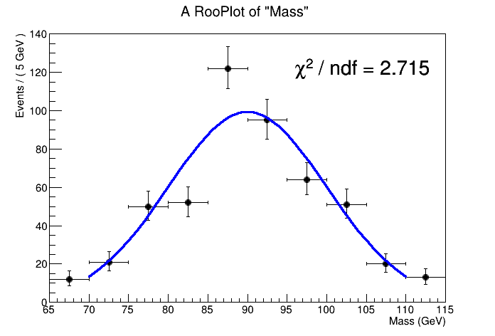
RooFit:
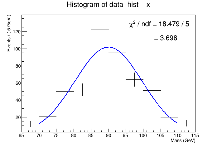
ROOT:
Can someone explain what is happening?
import ROOT
from ROOT import gROOT

from ROOT import RooFit
from ROOT import RooRealVar, RooGaussian
from ROOT import RooArgSet


def n_bins(range, bin_width):
    return int((range[1] - range[0]) / bin_width)


def dataset_to_hist(observable, dataset, name='data_hist'):
    roo_data_hist = ROOT.RooDataHist('h', '',
                                     ROOT.RooArgSet(observable), dataset)
    return roo_data_hist.createHistogram(name, observable)


def draw_RooPlot(observable, data, model, name, path=None, chi_square=True, fit_result=None):
    frame = observable.frame()
    data.plotOn(frame)
    model.plotOn(frame)
    canvas = ROOT.TCanvas()
    canvas.cd()
    frame.Draw()

    if chi_square:
        if fit_result:
            n_param = fit_result.floatParsFinal().getSize()
            reduced_chi_square = frame.chiSquare(n_param)
        else:
            reduced_chi_square = frame.chiSquare()
        print('chi^2 / ndf = {}'.format(reduced_chi_square))
        legend = ROOT.TLegend(0.5, 0.7, 0.89, 0.89)
        legend.SetBorderSize(0)  # no border
        legend.SetFillStyle(0)  # make transparent
        legend.Draw()
        legend.AddEntry(None,
                        '#chi^{2}' + ' / ndf = {:.3f}'.format(
                            reduced_chi_square), '')
        legend.Draw()

    canvas.Draw()
    if path:
        canvas.SaveAs(path + name + '.png')
        canvas.SaveAs(path + name + '.pdf')
        canvas.SaveAs(path + name + '.eps')
    else:
        canvas.SaveAs(name + '.png')
        canvas.SaveAs(name + '.pdf')
        canvas.SaveAs(name + '.eps')


def RooFit_chi_square(n_samples=1000):
    x_range = [65, 115]
    x = RooRealVar('x', 'Mass',
                   x_range[0], x_range[1], 'GeV')
    # Set binning to 5 GeV
    x.setBins(n_bins(x_range, 5))

    mean = RooRealVar('mean', 'mean', 90, 70, 100, 'GeV')
    width = RooRealVar('width', 'width', 10, 1, 100, 'GeV')
    model = RooGaussian('model', 'signal model',
                        x, mean, width)
    gen_data = model.generate(RooArgSet(x), n_samples)
    fit_result = model.fitTo(gen_data,
                             RooFit.Range(70, 110),
                             RooFit.Minos(ROOT.kTRUE),
                             RooFit.SumW2Error(ROOT.kTRUE),
                             RooFit.Save(ROOT.kTRUE))

    draw_RooPlot(x, gen_data, model,
                 'chi_square_RooFit_test', fit_result=fit_result)

    return dataset_to_hist(x, gen_data)


def draw_hist(hist, name, path=None, chi_square=True, fit_result=None):
    canvas = ROOT.TCanvas()
    canvas.cd()

    hist.SetStats(ROOT.kFALSE)
    hist.Draw()
    if chi_square and fit_result:
        chi_square = fit_result.Chi2()
        ndf = fit_result.Ndf()
        reduced_chi_square = chi_square / ndf
        legend = ROOT.TLegend(0.5, 0.7, 0.89, 0.89)
        legend.SetBorderSize(0)  # no border
        legend.SetFillStyle(0)  # make transparent
        legend.Draw()
        legend.AddEntry(None,
                        '#chi^{2}' + ' / ndf = {:.3f} / {}'.format(
                            chi_square, ndf), '')
        legend.AddEntry(None,
                        '             = {:.3f}'.format(reduced_chi_square), '')
        legend.Draw()

    canvas.Draw()
    if path:
        canvas.SaveAs(path + name + '.png')
        canvas.SaveAs(path + name + '.pdf')
        canvas.SaveAs(path + name + '.eps')
    else:
        canvas.SaveAs(name + '.png')
        canvas.SaveAs(name + '.pdf')
        canvas.SaveAs(name + '.eps')


def ROOT_chi_square(n_samples=1000, hist=None):
    x_range = [65, 115]

    if hist:
        gen_hist = hist
        gen_hist.SetLineColor(ROOT.kBlack)
    else:
        gen_hist = ROOT.TH1F('gen_hist', '', n_bins(x_range, 5),
                             x_range[0], x_range[1])

        model = ROOT.TF1('model', '[0]*exp(-0.5*((x-[1])/[2])**2)',
                         x_range[0], x_range[1])
        model.SetParameter(1, 90)
        model.SetParameter(2, 10)
        model.SetParameter(0, ROOT.TMath.Sqrt(2 * ROOT.TMath.Pi()) * 10)

        gen_hist.FillRandom('model', n_samples)

    fit_result = gen_hist.Fit('gaus', 'ILS', '', 70, 110)
    model = gen_hist.GetFunction('gaus')
    model.SetLineColor(ROOT.kBlue)

    chi_square = fit_result.Chi2()
    ndf = fit_result.Ndf()
    reduced_chi_square = chi_square / ndf
    print('chi^2 / ndf = {}'.format(reduced_chi_square))

    draw_hist(gen_hist,
              'chi_square_ROOT_test', fit_result=fit_result)

if __name__ == '__main__':
    gROOT.SetBatch(ROOT.kTRUE)

    n_samples = 500
    gen_hist = RooFit_chi_square(n_samples)
    ROOT_chi_square(n_samples, gen_hist)