Deconvolution of multiple peak structure

Mansi · June 9, 2020, 7:28pm

Hello,

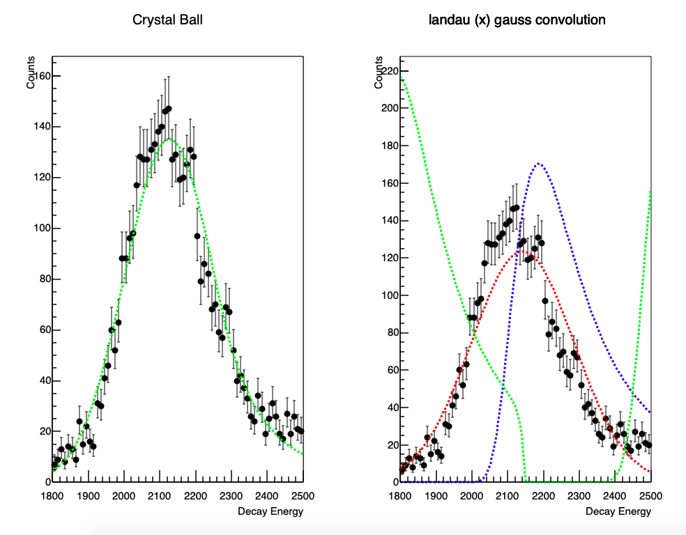
I have a histogram, which has different proton peaks- which are basically broad distributions. The high energy tailing in the peaks is due to the energy deposited by the betas in addition to the protons which are detected in the DSSD detector.
dssd-fit.pdf (37.7 KB)

Each peak visible in the histogram is actually a sum of two or three peaks, with known relative intensities.

For eg. The first dominant peak is sum of three peaks with supposed centroids at
1685 keV ->1878 channel (4% rel intensity)
1836 keV ->2029 channel ( 36% rel intensity)
1902 keV -> 2095 channel (100% rel intensity)

Im fitting this structure, as a total of three gaussians. But, I am unable to constrain the fits and reproduce the correct intensities. Also I end up having bad chi_square value.

The way I define the fitting routine is as follows -

 xpos[0]=1878.0;
 xpos[1]=2029.0;
 xpos[2]=2095.0;
 ypos[0] = decayEnergy->GetBinContent(xpos[0]);

 ypos[1] = decayEnergy->GetBinContent(xpos[1]);
 ypos[2] = decayEnergy->GetBinContent(xpos[2]);
 
 TCanvas *cEnergy = new TCanvas("cEnergy","cEnergy", 800,600);
 cEnergy->cd();
 
 cout<<"Ypos "<<ypos[0]<<endl;
 
 TF1 * F1 = new TF1("F1", "gaus",1446,2310); // Ep = 1685 peak -> 1878 channel# (3sigma= 144*3 = 432)
 TF1 * F2 = new TF1("F2", "gaus",1597,2461); // Ep = 1838 peak ->2029 channel
 TF1 * F3 = new TF1("F3", "gaus",1663,2527);// Ep = 1902 peak -> 2095 channel
 TF1 * total = new TF1("total", "gaus(0)+gaus(3)+gaus(6)",1440,2527); 
 
 F1->FixParameter(0,ypos[0]);
 F1->FixParameter(1,1878);
 F1->SetParameter(2,70);
 F1->SetLineColor(kGreen);
 // F1->FixParameter(0,90.0);
 decayEnergy->Fit("F1","SR");
 
 F2->FixParameter(0,ypos[1]);
 F2->FixParameter(1,2029);
 F2->SetParameter(2,70);
 F2->SetLineColor(kBlack);
 // F2->FixParameter(0,300.0);
 decayEnergy->Fit("F2","SR+");
 
 F3->FixParameter(0,ypos[2]);
 F3->SetParameter(1,2095);
 F3->FixParameter(2,70);
 F3->SetLineColor(kRed);
 //  F3->FixParameter(0,450.0);
 decayEnergy->Fit("F3","SER+");


 F1->GetParameters(&par[0]);
 F2->GetParameters(&par[3]);
 F3->GetParameters(&par[6]);


total->SetParameters(par);

 total->SetParLimits(1,1878,1920); // centroids
 total->SetParLimits(4,2030,2070);
 total->SetParLimits(7,2090,2130);
 total->SetParLimits(0,1,50); // heights
 total->SetParLimits(3,1,200);
 total->SetParLimits(6,1,200);
 total->SetParLimits(2,70,150); // sigmas
 total->SetParLimits(5,70,150);
 total->SetParLimits(8,70,150);
 
 
 total->SetLineColor(kMagenta);
 decayEnergy ->Fit("total", "SR+");
 total->Draw(" same");

Is there any better way to do this routine. Or is some other routine available within ROOT framework, which can be used

Thanks
Mansi

bellenot · June 9, 2020, 7:34pm

Maybe @moneta can give you some hints

Mansi · June 10, 2020, 1:34pm

yeah, sure!
Any help is needed

Wile_E_Coyote · June 10, 2020, 1:44pm

Attach data file.

Mansi · June 10, 2020, 2:42pm

decay-data.root (45.6 KB)
here is the data file.
DSSD-decay_Zn1 is the correct histogram.

Thanks

Wile_E_Coyote · June 10, 2020, 3:04pm

Three questions … when you say “three peaks, with known relative intensities” …

What about the “sigmas” of these three peaks … can one assume that they are exactly the same or can they be different?

By “relative intensities”, do you mean relative peaks’ heights or do you mean relative peaks’ areas?

Do you mean that the “relative intensities” are “fixed values” (i.e. exactly 4%, 36%, 100%) or do you want to “fit” them as “independent parameters”? In case you want to “fit” them, can you specify some “limits” for them?

Mansi · June 10, 2020, 3:29pm

Thanks,

The sigma values should be similar for them.
The sigma from the source calibration run is 70 keV. All the spectras energy calibrated
The resolution of the proton peaks, shown in the decay spectrum can also be affected by the energy deposited in the detector by the beta particles.

By relative intensities, I am referring to relative peak areas.

I would like to have to a total fit function reproducing the shape of the peaks and also the relative peak intensities for the individual peaks, which are summed up in these broad distributions.

Wile_E_Coyote · June 10, 2020, 6:52pm

I’m afraid I do not understand what you mean by e. g. “1902 keV -> 2095 channel (100% rel intensity)” and so on.

The key to success is to set “reasonable” initial values for all parameters of the fit function.

So, using the macro given below (zoom of the histogram from 1750 keV to 2550 keV), could you, please, tell me the means / positions of all three peaks and their sigmas (and their “limits”), first for the “100%” peak, then the “36%” peak and finally the “4%” peak.

{
  TFile *f = TFile::Open("decay-data.root");
  TH1D *h; f->GetObject("Correlator/DSSD_Decay+Clover/DSSD_Decay_!_Zn1", h);
  h->Sumw2(kTRUE); h->Rebin(10);
  Double_t xmin = 1750., xmax = 2550.;
  h->SetAxisRange(xmin, xmax, "X"); h->Draw();
}

Mansi · June 10, 2020, 7:04pm

These should be the centroids for the lines -

xpos[0]=1878.0; // for 4% rel intensity
xpos[1]=2029.0; // for 36% rel intensity
xpos[2]=2095.0; // for 100 % rel intensity

the limits for the sigma should be (70,150).

Wile_E_Coyote · June 10, 2020, 7:14pm

Well, I think this is not possible if their “sigma values should be similar”.
Looking at the histogram, it seems to me that the “100%” peak would need to be at least twice as broad as the “36%” peak.

Mansi · June 10, 2020, 7:19pm

yeah, on second thoughts,
The most 100% intense peak will have a bigger sigma value, as it might have Doppler effects, which might not be true for others.
But I do not have quantitative numbers?
what’s the best solution in that case ?

Wile_E_Coyote · June 10, 2020, 7:21pm

It seems to me that you need to talk to your colleagues.

Mansi · June 10, 2020, 7:27pm

ok thanks

Wile_E_Coyote · June 10, 2020, 7:39pm

Here’s what I tried:

{
  gStyle->SetOptStat(""); // "e" (Entries only) or "" (nothing at all)
  gStyle->SetOptFit(1112);
  TFile *f = TFile::Open("decay-data.root");
  TH1D *h; f->GetObject("Correlator/DSSD_Decay+Clover/DSSD_Decay_!_Zn1", h);
  h->Sumw2(kTRUE); h->Rebin(10);
  Double_t xmin = 1800., xmax = 2530.; // 1750. (1800.) ... (2530.) 2550.
  h->SetAxisRange(xmin - 100., xmax + 100., "X");
#if 0 /* 0 or 1 */
  h->Draw();
#else
  TF1 *f3 = new TF1("f3",
                    "[0] * (TMath::Gaus(x, [3], [6], 1) + ([1] / 100.) * TMath::Gaus(x, [4], [7], 1) + ([2] / 100.) * TMath::Gaus(x, [5], [8], 1))",
                    xmin, xmax);
  // 100% peak ... area, mean, sigma
  f3->SetParName(0, "a_100");
  f3->SetParameter(0, (100. / (100. + 36. + 4.)) * h->Integral(h->FindFixBin(xmin), h->FindFixBin(xmax), "width"));
  // f3->SetParLimits(0, , );
  f3->SetParName(3, "m_100");
  f3->SetParameter(3, 2095.);
  f3->SetParLimits(3, 2070., 2120.);
  f3->SetParName(6, "s_100");
  f3->SetParameter(6, 150.);
  f3->SetParLimits(6, 50., 300.);
  // 36% peak ... relative intensity, mean, sigma
  f3->SetParName(1, "r_36");
  f3->SetParameter(1, 36.); // 36%
  f3->SetParLimits(1, 15., 70.);
  f3->SetParName(4, "m_36");
  f3->SetParameter(4, 2029.);
  f3->SetParLimits(4, 2005., 2055.);
  f3->SetParName(7, "s_36");
  f3->SetParameter(7, 70.);
  f3->SetParLimits(7, 50., 150.);
  // 4% peak ... relative intensity, mean, sigma
  f3->SetParName(2, "r_4");
  f3->SetParameter(2, 4.); // 4%
  f3->SetParLimits(2, 1., 10.);
  f3->SetParName(5, "m_4");
  f3->SetParameter(5, 1878.);
  f3->SetParLimits(5, 1855., 1905.);
  f3->SetParName(8, "s_4");
  f3->SetParameter(8, 70.);
  f3->SetParLimits(8, 50., 150.);
  // f3->Print("V");
  h->Fit(f3, "LR"); // e.g. "R" or "LR"
#endif /* 0 or 1 */
}

Mansi · June 10, 2020, 7:49pm

Ok yeah !
to control the fit, the better initial guess will be needed.
As the chi_square per d.o.f is still quite high.

Mansi · June 10, 2020, 8:06pm

Ok Yes !
The shape of the peak is reproduced.

EXT PARAMETER STEP FIRST
NO. NAME VALUE ERROR SIZE DERIVATIVE
1 a_100 3.93824e+04 6.13286e+02 -2.20425e-01 -1.25536e-07
2 r_36 1.50000e+01 4.21237e-01 9.59837e-05** at limit **
3 r_4 1.00000e+00 6.09195e-02 -1.49706e-04** at limit **
4 m_100 2.12000e+03 1.04443e-01 8.09197e-06** at limit **
5 m_36 2.05500e+03 2.70480e-01 4.20801e-05** at limit **
6 m_4 1.85500e+03 1.14028e+01 8.52196e-06** at limit **
7 s_100 1.65410e+02 2.68250e+00 7.39277e-06 2.89610e-03
8 s_36 5.25073e+01 3.91393e+00 2.19523e-04 -3.17068e-06
9 s_4 1.50000e+02 2.10627e+00 -1.75943e-05** at limit **

But the limits will have to be played with ?

Wile_E_Coyote · June 10, 2020, 8:09pm

This is not a good fit at all.
You really need good initial values.
It is also possible that three Gauss functions are not able to describe your histogram well.
You need to talk to your colleagues.

BTW. Instead of the “LR” fit options, you can also try just “R” (the fit will still be bad and you will get many “** at limit **” warnings as well).

Mansi · June 10, 2020, 8:37pm

Ok, probably it will be better to use Landau convoluted with Gaussian distribution than just a Gaussian distribution.

But, not sure how to define a total function as sum of three peaks defined by Landau convoluted with Gaussian?

Wile_E_Coyote · June 10, 2020, 8:44pm

${ROOTSYS}/tutorials/fit/langaus.C

ROOT Forum -> Search -> langaus

Mansi · June 13, 2020, 8:32pm

Thanks,

@StephanH I wrote a new macro, defining the landau convolution with gauss. It seems to be working in TF1, but if I define using RooFit, I don’t get a good fit.
I plot the landau and gauss function independently, to estimate the initial parameter values.
But the convoluted landau and Gauss fit isn’t good.

Mansi

RooFitConv.C (5.3 KB)