Creating a TH2Poly

atha.stam · April 26, 2024, 9:22pm

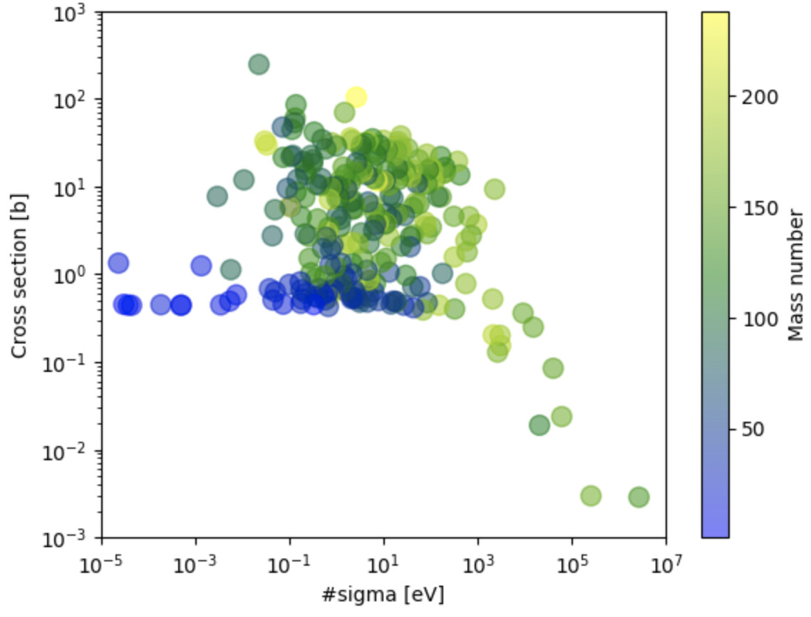
I have a TGraph that its point represents two nuclear properties for different nucleus.
I would like to create a TH2Poly and weigh the points by a 3rd nuclear property.

I create the TGraph from the first two columns (1st olumn is x and 2nd is y) from an ascii file that looks like that

2.650e+006 2.868e-003 135.00
2.540e+005 2.969e-003 157.00
6.090e+004 2.376e-002 155.00
4.014e+004 8.445e-002 149.00
2.060e+004 1.893e-002 113.00
1.517e+004 2.482e-001 151.00
9.200e+003 3.587e-001 151.00
3.080e+003 1.532e-001 196.00
3.000e+003 2.003e-001 184.00
2.650e+003 1.287e-001 164.00
2.300e+003 9.261e+000 168.00
2.150e+003 2.023e-001 199.00
2.090e+003 5.201e-001 176.00
9.540e+002 3.669e+000 191.00
7.350e+002 2.748e+000 152.00
6.590e+002 4.507e+000 167.00
6.000e+002 1.792e+000 161.00
5.630e+002 2.396e+000 180.00
5.610e+002 7.772e-001 174.00
4.180e+002 1.347e+001 123.00
3.730e+002 1.923e+001 177.00
3.250e+002 4.000e-001 143.00
3.200e+002 1.563e+000 187.00
3.120e+002 4.551e+000 153.00
2.060e+002 1.442e+001 152.00
2.020e+002 1.634e+001 115.00
1.940e+002 1.412e+001 162.00
1.800e+002 1.017e+000 83.00
1.684e+002 7.565e+000 147.00
1.650e+002 2.182e+001 124.00
1.520e+002 4.408e-001 190.00
1.450e+002 7.586e+000 103.00
1.240e+002 1.185e+001 163.00
1.120e+002 1.533e+001 185.00
1.110e+002 1.216e+001 193.00
1.050e+002 1.638e+001 169.00
1.040e+002 3.442e+000 150.00
9.865e+001 1.571e+001 197.00
9.100e+001 1.538e+001 109.00
8.500e+001 2.882e+000 154.00
8.500e+001 4.706e-001 76.00
8.500e+001 1.059e+001 131.00
8.400e+001 2.321e+001 178.00
8.000e+001 3.500e+000 186.00
7.640e+001 3.927e+000 187.00
6.940e+001 3.890e-001 174.00
6.470e+001 1.028e+001 165.00
6.000e+001 7.167e-001 50.00
5.720e+001 6.329e+000 138.00
5.700e+001 1.360e+001 147.00
5.600e+001 2.004e+001 160.00
5.180e+001 1.081e+001 74.00
4.860e+001 6.481e+000 171.00
4.360e+001 4.128e-001 35.00
4.300e+001 2.791e+000 158.00
4.200e+001 5.714e+000 145.00
4.200e+001 7.143e-001 77.00
4.100e+001 1.537e+001 179.00
3.790e+001 1.280e+001 186.00
3.760e+001 2.660e+000 107.00
3.718e+001 2.041e+000 59.00
3.300e+001 2.679e+001 156.00
3.000e+001 9.667e-001 115.00
2.900e+001 1.507e+001 133.00
2.800e+001 4.643e+000 82.00
2.750e+001 1.327e+001 195.00
2.720e+001 4.412e-001 45.00
2.500e+001 2.696e+001 189.00
2.400e+001 2.083e+000 111.00
2.350e+001 3.745e+001 176.00
2.340e+001 1.786e+001 159.00
2.310e+001 2.641e+001 175.00
2.100e+001 1.190e+001 129.00
2.070e+001 2.918e+001 182.00
2.050e+001 3.220e+001 181.00
2.000e+001 1.600e+001 99.00
2.000e+001 4.900e+000 105.00
1.960e+001 4.847e+000 166.00
1.900e+001 2.526e+001 162.00
1.870e+001 4.813e-001 142.00
1.820e+001 4.890e-001 53.00
1.710e+001 2.222e+001 173.00
1.600e+001 7.313e+000 87.00
1.590e+001 4.906e-001 50.00
1.500e+001 4.267e+000 73.00
1.450e+001 4.552e-001 62.00
1.400e+001 7.929e+000 95.00
1.330e+001 1.053e+000 55.00
1.304e+001 2.684e+000 180.00
1.300e+001 1.031e+001 164.00
1.200e+001 2.583e+001 113.00
1.150e+001 4.878e+000 80.00
1.150e+001 1.513e+000 141.00
1.140e+001 2.570e+001 170.00
1.140e+001 3.772e+000 203.00
1.130e+001 1.504e+001 130.00
1.100e+001 3.727e+000 110.00
1.100e+001 1.155e+001 79.00
1.010e+001 3.337e+001 183.00
1.000e+001 1.150e+001 192.00
8.930e+000 1.355e+000 139.00
8.400e+000 4.286e+000 154.00
8.300e+000 2.940e+001 108.00
7.840e+000 4.974e-001 48.00
7.800e+000 3.846e+000 201.00
7.370e+000 1.153e+001 232.00
7.100e+000 2.254e+001 99.00
6.800e+000 7.794e-001 124.00
6.800e+000 3.676e+000 67.00
6.500e+000 5.077e+000 132.00
6.300e+000 1.222e+001 136.00
6.200e+000 6.339e-001 43.00
6.200e+000 3.145e+000 78.00
6.200e+000 2.419e+001 127.00
5.900e+000 3.475e+001 121.00
5.800e+000 6.103e+000 170.00
5.800e+000 1.672e+001 135.00
5.100e+000 8.431e-001 137.00
5.000e+000 2.240e+000 100.00
4.900e+000 5.510e-001 51.00
4.890e+000 8.589e-001 202.00
4.710e+000 6.624e+000 71.00
4.700e+000 3.234e+001 188.00
4.600e+000 4.783e-001 58.00
4.500e+000 1.356e+001 75.00
4.500e+000 1.104e+000 63.00
4.100e+000 3.098e+001 123.00
3.660e+000 1.475e+001 198.00
3.600e+000 1.500e+000 144.00
3.500e+000 1.714e+001 126.00
3.400e+000 2.618e+001 122.00
3.400e+000 2.941e+000 102.00
3.400e+000 2.941e+001 101.00
3.150e+000 4.762e-001 70.00
2.900e+000 5.172e-001 60.00
2.850e+000 2.211e+000 176.00
2.740e+000 1.350e+001 168.00
2.700e+000 1.852e+001 81.00
2.680e+000 1.034e+002 238.00
2.590e+000 5.405e-001 56.00
2.500e+000 6.000e-001 61.00
2.500e+000 5.600e+000 148.00
2.480e+000 6.452e-001 57.00
2.400e+000 1.458e+001 148.00
2.300e+000 6.826e+000 117.00
2.250e+000 5.333e-001 54.00
2.200e+000 3.318e+001 158.00
2.200e+000 1.318e+000 119.00
2.200e+000 5.455e-001 49.00
2.200e+000 5.455e+000 112.00
2.170e+000 1.009e+000 65.00
2.100e+000 6.667e+000 97.00
2.100e+000 5.238e-001 39.00
2.000e+000 3.550e+001 198.00
2.000e+000 2.300e+000 192.00
2.000e+000 1.100e+001 134.00
1.700e+000 8.647e+000 184.00
1.700e+000 8.824e-001 47.00
1.680e+000 9.286e+000 69.00
1.550e+000 1.355e+001 125.00
1.520e+000 6.447e-001 64.00
1.500e+000 6.933e+001 156.00
1.460e+000 9.589e-001 41.00
1.440e+000 2.153e+000 194.00
1.400e+000 1.657e+001 146.00
1.280e+000 7.813e-001 89.00
1.280e+000 1.328e+000 58.00
1.240e+000 4.194e+000 91.00
1.210e+000 3.471e+000 102.00
1.200e+000 1.167e+001 150.00
1.150e+000 7.391e+000 93.00
1.100e+000 1.000e+001 108.00
1.040e+000 7.212e+000 126.00
1.040e+000 4.615e+000 86.00
1.010e+000 2.871e+001 112.00
9.800e-001 8.163e-001 72.00
9.500e-001 1.211e+000 142.00
8.800e-001 6.591e-001 44.00
8.700e-001 9.885e+000 84.00
8.500e-001 2.118e+000 66.00
8.000e-001 3.125e+001 172.00
7.700e-001 9.610e+000 160.00
7.600e-001 6.579e-001 52.00
7.600e-001 1.908e+000 64.00
7.400e-001 1.270e+000 46.00
7.200e-001 7.083e+000 196.00
7.120e-001 5.478e-001 207.00
7.000e-001 3.400e+000 144.00
6.800e-001 4.265e-001 42.00
6.610e-001 3.026e+000 204.00
6.600e-001 6.212e-001 40.00
6.100e-001 2.623e+000 80.00
6.000e-001 2.667e+001 104.00
5.900e-001 5.085e-001 46.00
5.700e-001 9.474e-001 140.00
5.300e-001 5.868e-001 23.00
5.100e-001 1.961e+000 74.00
5.000e-001 3.400e+001 96.00
4.800e-001 1.229e+001 85.00
4.500e-001 1.022e+001 132.00
4.330e-001 6.813e-001 37.00
4.100e-001 5.366e-001 40.00
4.000e-001 4.250e+000 136.00
3.800e-001 1.053e+001 78.00
3.600e-001 8.889e-001 138.00
3.600e-001 5.556e-001 54.00
3.400e-001 4.147e+001 114.00
3.326e-001 4.480e-001 1.00
3.200e-001 2.000e+001 104.00
3.150e-001 1.810e+001 106.00
2.900e-001 1.034e+000 130.00
2.900e-001 2.241e+001 96.00
2.650e-001 1.509e+000 134.00
2.600e-001 2.692e+000 136.00
2.310e-001 6.061e-001 27.00
2.270e-001 1.366e+001 110.00
2.200e-001 1.545e+001 118.00
2.200e-001 2.864e+000 92.00
2.150e-001 7.442e+000 128.00
1.990e-001 1.910e+001 100.00
1.900e-001 5.158e-001 25.00
1.800e-001 4.500e+000 122.00
1.790e-001 6.592e-001 50.00
1.770e-001 4.633e-001 28.00
1.720e-001 8.140e-001 31.00
1.500e-001 1.200e+001 76.00
1.400e-001 8.571e+000 120.00
1.400e-001 8.500e+001 116.00
1.340e-001 5.970e+001 124.00
1.300e-001 5.308e+001 98.00
1.200e-001 2.250e+001 87.00
1.150e-001 4.435e+001 114.00
1.100e-001 2.182e+001 84.00
1.070e-001 5.888e+000 30.00
1.040e-001 5.865e+000 205.00
1.010e-001 7.624e-001 29.00
9.100e-002 9.451e+000 70.00
7.500e-002 2.133e+001 116.00
7.500e-002 4.533e-001 14.00
7.200e-002 4.722e+001 68.00
5.100e-002 6.275e-001 24.00
4.990e-002 5.411e+000 94.00
4.550e-002 5.055e-001 22.00
4.400e-002 2.727e+000 82.00
3.820e-002 6.806e-001 26.00
3.380e-002 2.959e+001 209.00
3.060e-002 3.269e+001 206.00
2.290e-002 2.445e+002 96.00
1.100e-002 1.182e+001 90.00
7.600e-003 5.789e-001 9.00
5.500e-003 4.909e-001 11.00
3.530e-003 4.448e-001 12.00
1.370e-003 1.241e+000 13.00
5.190e-004 4.432e-001 2.00
5.000e-004 4.400e-001 10.00
1.900e-004 4.474e-001 16.00
4.540e-005 4.405e-001 7.00
3.850e-005 4.416e-001 6.00
3.100e-005 4.516e-001 3.00
2.400e-005 1.333e+000 15.00
3.000e-003 7.667e+000 86.00
5.800e-003 1.121e+000 88.00

I’m using the TGraph("file.dat", "%lg %lg %*lg") constructor and the plot looks as follows

My end goal is to weigh each point with the 3rd column of the ascii file. I think that using a TH2Poly is the best way, but I’m open to suggestions. The problem is that I’m not sure how to create it. I understand that I need to creat the bins first and then fill them. I think I can create the bins but it’s unclear how to properly fill Any tip is much appreciated!

#include "TH2Poly.h"

#include <vector>
#include <iostream>
#include <fstream>


using namespace std;

void createHistogramFromAsciiFile(const char* filename) {
    //Open the file
    ifstream file(filename);

    //Create vectors
    std::vector<double> X, Y, Z;
    double x, y, z;
    
    //Fill vectors
    while (file >> x >> y >> z) {
        X.push_back(x);
        Y.push_back(y);
        Z.push_back(z);
    }
    
    int size = (int) X.size();

    //Create a TH2Poly histogram
    double x_low = 1.e-5, x_up = 1.e7;
    double y_low = 1.e-3, y_up = 1.e3;
    double dx = 1.e-3;
    double dy = 1.e-3;
    
    TH2Poly *h = new TH2Poly("h", "h", x_low, x_up, y_low, y_up);

    // Fill the histogram
    for (int i=0; i< size; ++i)
        h->AddBin(size, X.data(), Y.data());
    
    //int bins = h->GetBins();
    cout << "Total bins = " << h->GetBins() << endl;

    //for (int i=0; i<bins; ++i)
        //h->Fill(i, Z[i]);

    // Draw the histogram
    h->Draw("colz");

}

Danilo · April 27, 2024, 5:18am

Hi,

Very nice plot! *
I have issues imagining what you are trying to achieve: can you perhaps paste a similar plot from a publication in order to show the visualisation you are trying to achieve?
Adding in the loop @couet

Cheers,
D

Could you share the full source to obtain it?

sfpate · April 27, 2024, 6:54pm

Why not use a regular TH2 and fill it with the weight?
Since you want to have log x and y axes, you might want to take the base10-logarithm of the x and y data, then create the TH2 with uniform bins from -5 to +7 (x-axis) and -3 to +3 (y-axis) and then fill.

TH2F *h2 = new TH2F("h2","",100,-5.,7.,100,-3.,3.);
loop over your data {  h2->Fill(TMath::Log10(x),TMath::Log10(y),weight); }

Something like that… I wonder if that is the effect you are trying to achieve.

couet · April 29, 2024, 7:17am

Yes, a regular TH2F is better in that case.

atha.stam · April 29, 2024, 2:28pm

Hello!

Each point represents a nucleus.
The x is capture cross section and the the y resonance integral.
I want to weigh each point with the mass number.
That way you can essentially see that the higher the mass number, the higher the cross section and the resonance integral, with a few exceptions. These exceptions should be nicely visualized if I weigh each point with the mass number.
This graph doesn’t exist in a publication, as far as I know.

To get the plot, you have to do a literature search.
The values I pasted include the data.

atha.stam · April 29, 2024, 2:34pm

Hello!
Thanks for the suggestion!

The reason is that each point should be a single bin.
I know I can have a variable bin but I can’t think of what the low edges will look like in that case.
Also, it’s not clear what the width of these bins should be if I make it a TH2
And probably if I do that, I think I’ll end up in many empty bins.

I just thought TH2Poly is the best object for what I’m trying to achieve.

sfpate · April 29, 2024, 2:55pm

I am beginning to understand. I think this is not appropriate for any sort of histogram, however. This is a kind of “scatter plot”, in my mind.

What if the mass number determined the color of the point? You could establish a color scale from the range of masses. Then large masses (bluish?) would be distinguished from low masses (reddish?). Before you plot each point, you determine and set the color of the point.

I hope that suggestion is helpful.

atha.stam · April 29, 2024, 3:21pm

Hello.

Yes, that would make more sense.
I can do a similar thing in python, but I’m just trying to do it with root.

For reference here’s the python code and the output
Note I’m a complete newbie in Python and did that to learn.

import numpy as np
import matplotlib.pyplot as plt
from matplotlib.colors import LinearSegmentedColormap

# Define the colors from the ROOT palettes
kBird_colors = [(0, "#0000FF"), (0.5, "#008000"), (1, "#FFFF00")]  # Blue to Green to Yellow
kGreyScale_colors = [(0, "#000000"), (1, "#FFFFFF")]  # Black to White
kRainBow_colors = [(0, "#FF0000"), (0.33, "#FFFF00"), (0.67, "#00FF00"), (1, "#0000FF")]  # Red to Yellow to Green to Blue

# Create the custom colormaps
kBird_cmap = LinearSegmentedColormap.from_list("kBird", kBird_colors)
kGreyScale_cmap = LinearSegmentedColormap.from_list("kGreyScale", kGreyScale_colors)
kRainBow_cmap = LinearSegmentedColormap.from_list("kRainBow", kRainBow_colors)

# Read data from file and extract energy (S), cross section (I), and weight (A)
data_file = '../data.txt'  # Update with your file name
with open(data_file, 'r') as file:
    lines = file.readlines()

S, I, A = [], [], []
for line in lines:
    values = line.split()
    S.append(float(values[0]))
    I.append(float(values[1]))
    A.append(float(values[2]))

# Convert to numpy arrays
S = np.array(S)
I = np.array(I)
A = np.array(A)

# Plotting the scatter plot with colored points
scatter = plt.scatter(S, I, s=100, c=A, cmap=kBird_cmap, alpha=0.5)
plt.colorbar(scatter, label='Mass number')
plt.xlabel('#sigma [eV]')
plt.ylabel('Cross section [b]')
plt.xscale('log')
plt.yscale('log')
plt.xlim(1e-5, 1e7)
plt.ylim(1e-3, 1e3)
plt.show()

sfpate · April 29, 2024, 5:12pm

Lovely!

I think you should have a look here: