Bifurcation Diagram

Sisisan · June 1, 2017, 11:32pm

Hi All,

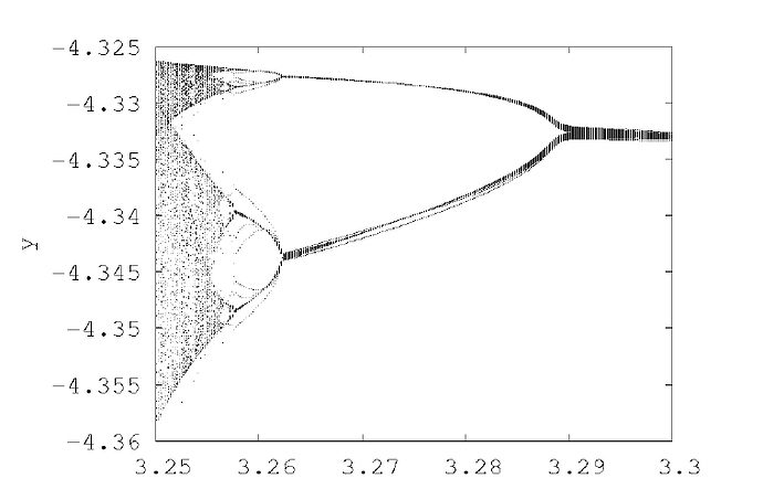
Do you have any idea about how to plot a bifurcation diagram in 3D nonlinear differential equations ?
I mean that which computational method do i need to use to plot a bifurcation diagram ?

Could it be such that the first is to use the newton-raphson method with gaussian elimination to find the roots of equations , then the second is to draw a bifurcation diagram which consists of a control parameter versus one of the roots which found with the method ?

I tried to draw the diagram with the method i mentioned above. As a control parameter varies, i found the roots, then i plotted the diagram one of roots versus a control parameter. However, i didn’t get it.

My script is as in the following ;

//The Hindmarsh_Rose Neuronal Model '84
//Firstly, Finds the roots of the equations via Newton's Raphson and Gaussian-Elimination
//Then, as a control parameter varies, draw a bifurcation diagram which consists of a control parameter versus one of the roots

#include <iostream>
#include <tuple>
#include <TMath.h>
#include <TH2D.h>
#include <TCanvas.h>
#include <fstream>

Int_t size = 3;
Int_t n =3;


using namespace std;


Double_t  f1(Double_t &x, Double_t &y, Double_t &z,Double_t &u) {

  Double_t f1;

  f1 = y+3.0*pow(x,2)-pow(x,3)-z+u;

  return f1;

}

Double_t  f2(Double_t &x, Double_t &y) {

  Double_t f2;

  f2 = 1.0-5.0*pow(x,2)-y;

  return f2;

}

Double_t  f3(Double_t &x, Double_t &z) {

  Double_t f3;

  f3 = 0.001*(4.0*(x-(-1.6180))-z);

  return f3;

}

tuple <Double_t, Double_t, Double_t, Double_t, Double_t, Double_t, Double_t, Double_t, Double_t> J(Double_t &x, Double_t &y, Double_t &z) {

  Double_t j1[3] = {(-3.0*pow(x,2)+6.0*x),(1.0),(-1.0)};
  Double_t j2[3] = {(-10.0*x),(-1.0),(0)};
  Double_t j3[3] = {(0.004),(0.0),(-0.001)};

  return make_tuple(j1[0],j1[1],j1[2],j2[0],j2[1],j2[2],j3[0],j3[1],j3[2]);

}


tuple <Double_t, Double_t, Double_t>  NaiveGaussianElimination(Double_t a[3][3], Double_t b[3]) {


  Double_t factor,sum;
  Int_t k,i,j;

 Double_t x[3];

  for(k=0; k<n-1; k++) {

    for(i=k+1; i<n; i++) {

      factor = a[i][k]/a[k][k];

      for(j=k+1;  j<n; j++) {

        a[i][j] = a[i][j] - factor * a[k][j];

      }

      b[i] =  b[i] - factor * b[k];

    }

  }

  for(i=2; i<n; i++) {
 x[i] = b[i] / a[i][i];

  }


  for(i=n-1; i>-1; i--) {

    sum = b[i];

    for(j=i+1; j<=n; j++) {

      sum = sum - a[i][j] * x[j];

    }

    x[i] = sum / a[i][i];

  }

  return make_tuple(x[0],x[1],x[2]);
}

void NewtonsRaphsonForNonlinear3D() {

  TH2D *h1 = new TH2D("h1","Bifurcation Diagram",10000,2,3,10000,-3,-4);

  Int_t N=5;
  Double_t j00,j01,j02,j10,j11,j12,j20,j21,j22;
  Double_t a[3][3],b[3],c[3];
  Double_t x,y,z,p,r,s,u,f,g,h;
  Double_t time;

  x = 0.1;
  y = 0.1;
  z = -0.1;
  u = 1.0;
  time = 0.0004;


  while(u<=5.0) {
  x = 0.1;
        y = 0.1;
        z = -0.1;

    for(Int_t i=0; i<N; i++) {

      //Computing J(x(0))y(0) = −F(x(0))
      b[0] = f1(x,y,z,u);
      b[1] = f2(x,y);
      b[2] = f3(x,z);

      tie(a[0][0],a[0][1],a[0][2],a[1][0],a[1][1],a[1][2],a[2][0],a[2][1],a[2][2])=J(x,y,z);


      for(Int_t j=0; j<3; j++) {

        c[j] = (-1.0)*b[j];

      }
 tie(p,r,s)=NaiveGaussianElimination(a,c);

      f=x;
      g=y;
      h=z;

      x += p;
      y += r;
      z += s;

      /*      cout<<f-x<<"\t";
      cout<<g-y<<"\t";
      cout<<h-z<<"\t";
      */

      cout<<setprecision(8);
      cout<<setw(20);
      //      cout<<x<<setw(20)<<y<<setw(20)<<z<<setw(20)<<endl;

    }
   cout<<x<<setw(20)<<y<<setw(20)<<z<<setw(20)<<endl;
     u += time;
     h1->Fill(u,y);

  }
  h1->Draw();

}

Also, i tried to draw the diagram and solve the equations with Runge-Kutta method as the control parameter varies. But again, i didn’t achieve it!

This script is as in the following;

include <iostream>
#include <TGraph.h>
#include <TCanvas.h>
#include <fstream>
#include <TMath.h>

using namespace std;


void HR_Bifurcation_R() {

  TCanvas *c1 = new TCanvas("c1","Hindmarsh-Rose Model",800,600);

  TH2D *h1 = new TH2D("h1","r vs  y(t)",10,0,0.005,10,-2,2);

  Int_t N = 100;
  Double_t a,b,c,d,s,x0,u;
  Double_t x,y,z,t,r;
  Double_t k1,k2,k3,k4,l1,l2,l3,l4,m1,m2,m3,m4;
  Double_t h,p;


  //initial conditions                                                                                                                                                              \

  a = 1.0;
  b = 3.0;
  c = 1.0;
  d = 5.0;
  x0 = -1.6180;
  u = 3.25;
  s = 4.0;
  t = 0.0;
  r = 0.0;
  h = 0.001;
  p = 0.00005;

  Int_t i;


  while(r<=0.005) {

    x = 0.1;
    y = 0.1;
    z = 0.1;

    for (i=0; i<N; i++) {

      //Runge-Kutta Method
      k1 = ((-a*(TMath::Power(x,3)))+b*(TMath::Power(x,2))+y-z+u);
      l1 = (c-d*(TMath::Power(x,2))-y);
      m1 = (r*(s*(x-x0)-z));

      k2 = ((-a*(TMath::Power((x+0.5*k1*h),3)))+b*(TMath::Power((x+0.5*k1*h),2))+(y+0.5*l1*h)-(z+0.5*m1*h)+u);
      l2 = (c-d*(TMath::Power((x+0.5*k1*h),2))-(y+0.5*l1*h));
      m2 = (r*(s*((x+0.5*k1*h)-x0)-(z+0.5*m1*h)));

      k3 = ((-a*(TMath::Power((x+0.5*k2*h),3)))+b*(TMath::Power((x+0.5*k2*h),2))+(y+0.5*l2*h)-(z+0.5*m2*h)+u);
      l3 = (c-d*(TMath::Power((x+0.5*k2*h),2))-(y+0.5*l2*h));
      m3 = (r*(s*((x+0.5*k2*h)-x0)-(z+0.5*m2*h)));

      k4 = ((-a*(TMath::Power((x+k3*h),3)))+b*(TMath::Power((x+k3*h),2))+(y+l3*h)-(z+m3*h)+u);
      l4 = (c-d*(TMath::Power((x+k3*h),2))-(y+l3*h));
      m4 = (r*(s*((x+k3*h)-x0)-(z+m3*h)));

      x = x + ((k1+2*(k2+k3)+k4)/6)*h;
      y = y + ((l1+2*(l2+l3)+l4)/6)*h;
      z = z + ((m1+2*(m2+m3)+m4)/6)*h;


      t += h;

     cout<<x<<"\t"<<y<<"\t"<<z<<"\t"<<t<<"\t"<<r<<endl;
     h1->Fill(r,y);

    }

    r += p;

  }

  c1->cd();
  h1->SetTitle("Bifurcation Diagram of HR Model");
  h1->GetXaxis()->SetTitle("r");
  h1->GetYaxis()->SetTitle("y(t) - The exchange of Ions");
  h1->Draw();

}

Thanks a lot,
Cheers,
Ersel

couet · June 2, 2017, 7:08am

Looking how these kind of diagrams look like I have the feeling that TH2D is not the best object to hold them. And surely the default drawing option which draws random points in bins is misleading.

My guess is that a TGraph drawn wit option “AP” will better reflect the pictures I saw of these kind of diagrams. I tried to modify you macro doing:

  TGraph *g = new TGraph();

instead of:

  TH2D *h1 = new TH2D("h1","r vs  y(t)",10,0,0.005,10,-2,2);

then:

     g->SetPoint(i,r,y);

instead of:

     h1->Fill(r,y);

and finally:

g->Draw("apl");

instead of:

  h1->Draw();

but all what I get is a vertical line at 0.005. I am completely ignorant of these kind of diagrams so it is difficult to help you further . But I feel the TGraph approach is the right one.

behrenhoff · June 2, 2017, 7:44am

Unfortunately I can’t help with your problem, but I’ve got a suggestion to your code.

The excessive use of tuple/tie makes the code hard to read. I’d use it only for up to 2 values - or for template metaprogramming where you sometimes need variable many things in a tuple (-> variadic template).

I am looking especially at the J function. As an alternative, you can do:

using M3x3 = std::array<std::array<Double_t, 3>, 3>;

M3x3 J(Double_t &x, Double_t &y, Double_t &z) {
  using v3 = std::array<Double_t, 3>;
  v3 j1 = {(-3.0*pow(x,2)+6.0*x),(1.0),(-1.0)};
  v3 j2 = {(-10.0*x),(-1.0),(0)};
  v3 j3 = {(0.004),(0.0),(-0.001)};

  return {{{j1}, {j2}, {j3}}}; // much shorter, you dont need to repeat j1[0,1,2] ...
}

// signature of NaiveGaussianElimination becomes:
tuple <Double_t, Double_t, Double_t>  NaiveGaussianElimination(M3x3 &a, Double_t b[3])

// and in NewtonsRaphsonForNonlinear3D, you simply define a as
M3x3 a;

// when assigning from J, get rid of the tie!
a=J(x,y,z);

Next step is to replace all your 3-element tuples<double,doule,double> with a v3 type.

And obvious question: what are the parameters y and z for in J? You are not using them.

Sisisan · June 2, 2017, 2:03pm

Thank you Wolf for regulating my script, it works well. But the essential problem still continue…

Thanks for your help Olivier. But it didn’t work on TGraph,

I want to plot something like this;

couet · June 6, 2017, 9:04am

I am sorry it didn’t help. My point was just to say that what you want looks like a an x,y plot where each x,y pair is displayed as a dot. If it is the case, there is two ways to draw such things in ROOT either using TGraph with option P or drawing a two variables plot with TTree using the default drawing option

system · June 20, 2017, 9:04am

This topic was automatically closed 14 days after the last reply. New replies are no longer allowed.