Hello,
I’m trying to fit a distribution - a mass distribution - with a polynomial and a bump modeled as a gaussian. But the the 2nd and 3rd degree terms seem “locked” at 0 i.e. the best fit seems to be a line. (I’ve explicitly set setConstant(kFALSE) for these variables so I’m pretty sure I’m not locking them trivially. Also I include the Minuit output below.)
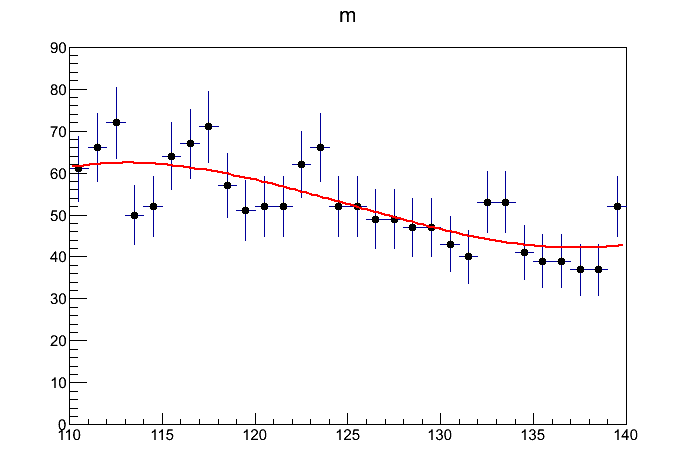
In addition, the line definitely doesn’t seem to be the best fit line that one would expect by eye.
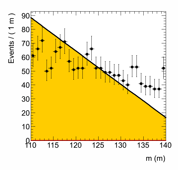
I attach 2 plots - the first one is the ‘problem’ output. The second one I get using “plain root” - meaning not roofit - and a binned histogram and the TH1F::Fit(TF1) functionality, just as a check. Assuming that whomever reads this might have lxplus access, I’ve put both scripts at ~scherzer/public/rooFitIssue. The RooFit script is rf.C and the other one is pr.C (plain root.)
I sort of suspect that maybe it has something to do with the step size that the parameters are varied with.(?) Because the bin fit returns values for these coefficients of O(10e-5) and maybe roofit doesn’t naturally slice that fine? I don’t know if that’s possible.
(I’m aware this is a pretty simple operation but somewhere I’m erroring!)
Thanks for the help. At the very end after the Minuit outputs I copy-paste sections from the script.)
Best regards,
Max
Minuit output using RooFit, bg2 = quadratic coefficient in background polynomial
3 bg1 -4.79426e-02 4.79426e-02 -0.00000e+00 0.00000e+00
4 bg2 0.00000e+00 8.41471e-02 -0.00000e+00 0.00000e+00
5 bg3 0.00000e+00 8.41471e-02 -0.00000e+00 0.00000e+00
Minuit output using Root’s binned fitter, in “L” mode
2 p1 -2.42284e-02 7.47834e-03 -5.67718e-05 3.74519e-02
3 p2 1.28411e-04 4.62344e-04 -5.37500e-06 -4.57879e+00
4 p3 5.48287e-05 5.04019e-05 2.24302e-07 6.20138e+00
====where I define the polynomial pdf====
//RooRealVar bg0(“bg0”, “bg0”, 1.0);
RooRealVar bg1(“bg1”, “bg1”, 0.0, -1.0/10.0, +1.0/10.0);
RooRealVar bg2(“bg2”, “bg2”, 0.0, -1.0/10.0, +1.0/10.0);
RooRealVar bg3(“bg3”, “bg3”, 0.0, -1.0/10.0, +1.0/10.0);
//bg0.setConstant(kTRUE); bg1.setConstant(kFALSE);
bg2.setConstant(kFALSE);
bg3.setConstant(kFALSE);
//RooChebychev mass_bg_pdf(“mass_bg_pdf”, “mass_bg_pdf”, m, RooArgList(bg1, bg2, bg3)); RooGenericPdf mass_bg_pdf(“mas_bg_pdf”, “bg3*(m-126.0)(m-126.0)(m-126.0) + bg2*(m-126.0)(m-126.0) + bg1(m-126.0) + 1.0”, RooArgList(m, bg1, bg2, bg3));
====where I put it together to make the final fit model====
RooRealVar Nggf(“Nggf”, “Nggf”, 0.025sampleSize, 0.0sampleSize, +0.05sampleSize);
RooRealVar Nbg( “Nbg”, “Nbg”, 0.975sampleSize, 0.0sampleSize, +1.00sampleSize); Nggf.setConstant(kFALSE);
Nbg.setConstant(kFALSE);
RooAddPdf model(“model”, “model”, RooArgList(mass_ggf_pdf, mass_bg_pdf), RooArgList(Nggf, Nbg)); RooFitResult* result; result = model.fitTo(*rds);