Access toy datasets generated by RooStat::FrequentistCalculator

Hello,
I’m trying to derive an upper upper limit on a signal with a hypothesis test using the profile likelihood test statistics. The fit model is very simple (flat background plus Gaussian signal). As the observed background is very small (only O(1) event) I am interested in looking at the toy data generated during the use of FrequentistCalculator. In particular, I want to know how many events are generated for each toy data set.
What does RooStats/RooFit do when no event is generated (for mean=1 event in 36% of all cases)?
Thanks,

Lukas

Hi,

The standard profile likelihood test statistics allows to store a more detailed output which include the fit parameter results, however this does not include the toy MC data (e.g. number of events generated).
However you can customise the FrequentistCalculator to use more test statistics and use in addition the NumEventTestStat class, so you can retrieve and histogram that information

Best Regards

Lorenzo

Hi Lorenzo,

thank you for your answer. Could you give me an example of how I can access that information with the NumEventsTestStat class? I created a minimal working example of my problem in python (see below). Unfortunately the method GetDetailedOutput() on the NumEventsTestStat object returns a Null-pointer.

On a more general note: can you (or anyone else) tell me what RooStats does with generated empty toy data sets? In RooFit with the RooMCStudy I found that these simply do not get fitted. In case of a very small background there should be a large fraction of empty data sets!
Thanks,

Lukas

#!/usr/bin/env python

import ROOT
from ROOT import RooFit as RF
from ROOT import RooStats as RS

NTOYS = 1000


# ROOT settings
ROOT.Math.MinimizerOptions.SetDefaultMinimizer('Minuit2')

# Workspace
w = ROOT.RooWorkspace('w')

# Observable
E = w.factory('E[0.,100.]')

# Constrained parameters and constraint PDF
mean = w.factory('mean[50.,49.,51.]')
mean_obs = w.factory('mean_obs[50.,49.,51.]')
mean_obs.setConstant(True)
mean_err = w.factory('mean_err[0.2]')
cpdf_mean = w.factory('Gaussian::cpdf_mean(mean,mean_obs,mean_err)')

sigma = w.factory('sigma[1.,0.5,1.5]')
sigma_obs = w.factory('sigma_obs[1.,0.5,1.5]')
sigma_obs.setConstant(True)
sigma_err = w.factory('sigma_err[0.1]')
cpdf_sigma = w.factory('Gaussian::cpdf_sigma(sigma,sigma_obs,sigma_err)')

# Signal
n_sig = w.factory('n_sig[0.,0.,10.]')
pdf_sig = w.factory('Gaussian::pdf_sig(E,mean,sigma)')

# Background
n_bkg = w.factory('n_bkg[10.,0.,50.]')
pdf_bkg = w.factory('Polynomial::pdf_bkg(E,{})')

# PDF
pdf_sum = w.factory('SUM::pdf_sum(n_sig*pdf_sig,n_bkg*pdf_bkg)')
pdf_const = w.factory('PROD::pdf_const({pdf_sum,cpdf_mean,cpdf_sigma})')

# ModelConfig
mc = RS.ModelConfig('mc', w)
mc.SetPdf( pdf_const )
mc.SetParametersOfInterest( ROOT.RooArgSet(n_sig) )
mc.SetObservables( ROOT.RooArgSet(E) )
mc.SetConstraintParameters( ROOT.RooArgSet(mean, sigma) )
mc.SetNuisanceParameters( ROOT.RooArgSet(mean, sigma, n_bkg) )
mc.SetGlobalObservables( ROOT.RooArgSet(mean_obs, sigma_obs) )

# Create toy data
data = pdf_sum.generate(ROOT.RooArgSet(E), RF.Name('data'), RF.Verbose(True), RF.Extended())
ROOT.RooAbsData.setDefaultStorageType(ROOT.RooAbsData.Vector)
data.convertToVectorStore()

# Print workspace
w.Print()

# Get RooStats ModelConfig from workspace and save it as Signal+Background model
sbModel = mc
poi = sbModel.GetParametersOfInterest().first()
poi.setVal(1.)
sbModel.SetSnapshot(ROOT.RooArgSet(poi))

# Clone S+B model, set POI to zero and set as B-Only model
bModel = mc.Clone()
bModel.SetName('mc_with_poi_0')
poi.setVal(0.)
bModel.SetSnapshot(ROOT.RooArgSet(poi))

RS.UseNLLOffset(True)

hc = RS.FrequentistCalculator(data, bModel, sbModel)
hc.SetToys(int(NTOYS), int(NTOYS/2.))
hc.StoreFitInfo(True)
hc.UseSameAltToys()

# Test statistics a: profile likelihood
profll = RS.ProfileLikelihoodTestStat(sbModel.GetPdf())
profll.EnableDetailedOutput()
profll.SetLOffset(True)
profll.SetMinimizer('Minuit2')
profll.SetOneSided(False)
profll.SetPrintLevel(0)
profll.SetStrategy(2)
profll.SetAlwaysReuseNLL(True)
profll.SetReuseNLL(True)

# Test statistics b
eventstat = RS.NumEventsTestStat(sbModel.GetPdf())

# Choose test statistics
teststat = profll
# teststat = eventstat

toymcs = hc.GetTestStatSampler()
toymcs.SetTestStatistic(teststat)
toymcs.SetUseMultiGen(True)

# HypoTestInverter
calc = RS.HypoTestInverter(hc)
calc.SetConfidenceLevel(0.90)
calc.UseCLs(True)
calc.SetVerbose(False)
calc.SetFixedScan(6, 0., 5., False)
hypotestresult = calc.GetInterval()

# Plot HypoTestInverter result
canvas = ROOT.TCanvas()
plot = RS.HypoTestInverterPlot('hypotest_inverter', 'hypotest inverter', hypotestresult)
plot.MakePlot()
plot.MakeExpectedPlot()
plot.Draw('CLB2CL')

# Print information
hc.GetFitInfo().Print('v')
teststat.GetDetailedOutput().Print('v')

Hi,

The Evaluate() method of NumEventsTestStat will return the number of events in the data set and this information should be stored in the detailed output.
Unfortunately I don;t have an example for this, but I could try to make one when I find some time.
Your code seems fine, apart from the fact that you need to define multiple test statistics as this:

toymcs.SetTestStatistic(profile,0)
toymcs.SetTestStatistic(eventstat,1)

For the other questions, I think in case of zero events no fit will be performed and probably a default value will be returned for the test statistics, but this needs to be checked. RooStats will not do anything peculiar, will create an empty data set and then depends on RooFit and the test statistics used on the handling of this empty data set

Lorenzo

Hi Lorenzo,

thank you for the quick reply. I implemented the two lines. Unfortunately, the pointer returned by

eventstat.GetDetailedOutput()

is empty and no information is available. Looking at RooStats::TestStatistics it seems like this method is not implemented for RooStats::NumEventsTestStat:

return detailed output: for fits this can be pulls, processing time, ... The returned pointer will not loose validity until another call to Evaluate.

Reimplemented in RooStats::SimpleLikelihoodRatioTestStat, RooStats::RatioOfProfiledLikelihoodsTestStat, RooStats::ProfileLikelihoodTestStat, and RooStats::MinNLLTestStat.

UPDATE:
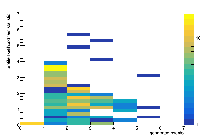
It did work after all. The information from the second test statistic NumEventsTestStat about how many events were generated is stored (additionally to the fit information from the ProfileLikelihoodTestStat) in the datasets which are returned by HypoTestResult::GetNullDetailedOutput() and HypoTestResult::GetAltDetailedOutput(). With this I can get easily retrieve and plot the distributions. For completeness the full code below.
Thank you very much for your help! Now I need to still find out what happens when the number of background events goes towards zero …

Lukas

#!/usr/bin/env python

import ROOT
from ROOT import RooFit as RF
from ROOT import RooStats as RS

NTOYS = 1000


# ROOT settings
ROOT.Math.MinimizerOptions.SetDefaultMinimizer('Minuit2')

# Workspace
w = ROOT.RooWorkspace('w')

# Observable
E = w.factory('E[0.,100.]')

# Constrained parameters and constraint PDF
mean = w.factory('mean[50.,49.,51.]')
mean_obs = w.factory('mean_obs[50.,49.,51.]')
mean_obs.setConstant(True)
mean_err = w.factory('mean_err[0.2]')
cpdf_mean = w.factory('Gaussian::cpdf_mean(mean,mean_obs,mean_err)')

sigma = w.factory('sigma[1.,0.5,1.5]')
sigma_obs = w.factory('sigma_obs[1.,0.5,1.5]')
sigma_obs.setConstant(True)
sigma_err = w.factory('sigma_err[0.1]')
cpdf_sigma = w.factory('Gaussian::cpdf_sigma(sigma,sigma_obs,sigma_err)')

# Signal
n_sig = w.factory('n_sig[0.,0.,10.]')
pdf_sig = w.factory('Gaussian::pdf_sig(E,mean,sigma)')

# Background
n_bkg = w.factory('n_bkg[10.,0.,50.]')
pdf_bkg = w.factory('Polynomial::pdf_bkg(E,{})')

# PDF
pdf_sum = w.factory('SUM::pdf_sum(n_sig*pdf_sig,n_bkg*pdf_bkg)')
pdf_const = w.factory('PROD::pdf_const({pdf_sum,cpdf_mean,cpdf_sigma})')

# ModelConfig
mc = RS.ModelConfig('mc', w)
mc.SetPdf( pdf_const )
mc.SetParametersOfInterest( ROOT.RooArgSet(n_sig) )
mc.SetObservables( ROOT.RooArgSet(E) )
mc.SetConstraintParameters( ROOT.RooArgSet(mean, sigma) )
mc.SetNuisanceParameters( ROOT.RooArgSet(mean, sigma, n_bkg) )
mc.SetGlobalObservables( ROOT.RooArgSet(mean_obs, sigma_obs) )

# Create toy data
data = pdf_sum.generate(ROOT.RooArgSet(E), RF.Name('data'), RF.Verbose(True), RF.Extended())
ROOT.RooAbsData.setDefaultStorageType(ROOT.RooAbsData.Vector)
data.convertToVectorStore()

# Print workspace
w.Print()

# Get RooStats ModelConfig from workspace and save it as Signal+Background model
sbModel = mc
poi = sbModel.GetParametersOfInterest().first()
poi.setVal(1.)
sbModel.SetSnapshot(ROOT.RooArgSet(poi))

# Clone S+B model, set POI to zero and set as B-Only model
bModel = mc.Clone()
bModel.SetName('mc_with_poi_0')
poi.setVal(0.)
bModel.SetSnapshot(ROOT.RooArgSet(poi))

RS.UseNLLOffset(True)

hc = RS.FrequentistCalculator(data, bModel, sbModel)
hc.SetToys(int(NTOYS), int(NTOYS/2.))
hc.StoreFitInfo(True)
hc.UseSameAltToys()

# Test statistics a: profile likelihood
profll = RS.ProfileLikelihoodTestStat(sbModel.GetPdf())
profll.EnableDetailedOutput()
profll.SetLOffset(True)
profll.SetMinimizer('Minuit2')
profll.SetOneSided(False)
profll.SetPrintLevel(0)
profll.SetStrategy(2)
profll.SetAlwaysReuseNLL(True)
profll.SetReuseNLL(True)

# Test statistics b
eventstat = RS.NumEventsTestStat(sbModel.GetPdf())

toymcs = hc.GetTestStatSampler()
toymcs.SetTestStatistic(profll,0)
toymcs.SetTestStatistic(eventstat,1)
toymcs.SetUseMultiGen(True)

# HypoTestInverter
calc = RS.HypoTestInverter(hc)
calc.SetConfidenceLevel(0.90)
calc.UseCLs(True)
calc.SetVerbose(False)
calc.SetFixedScan(6, 0., 5., False)
hypotestresult = calc.GetInterval()

# Plot HypoTestInverter result
c1 = ROOT.TCanvas()
plot = RS.HypoTestInverterPlot('hypotest_inverter', 'hypotest inverter', hypotestresult)
plot.MakePlot()
plot.MakeExpectedPlot()
plot.Draw('CLB2CL')

# Print information
hc.GetFitInfo().Print('v')

# Distribution of generated events for one hypothesis test
result = hypotestresult.GetResult(1)

h_null = ROOT.TH1I('h_null', 'generated events for null hypothesis', 50, 0, 50)
h_null.SetLineColor(ROOT.kBlue)
data_null = result.GetNullDetailedOutput()
for i in range( int(NTOYS) ):
    h_null.Fill( data_null.get(i).find('mc_TS1').getVal() )
    
h_alt = ROOT.TH1I('h_alt', 'generated events for alt hypothesis', 50, 0, 50)
h_alt.SetLineColor(ROOT.kRed)
data_alt = result.GetAltDetailedOutput()
for i in range( int(NTOYS/2) ):
    h_alt.Fill( data_alt.get(i).find('mc_with_poi_0_TS1').getVal() )

# Plot    
c2 = ROOT.TCanvas()
h_null.Draw()
h_alt.Draw('SAME')

I did a simple test and set the number of background events in the actual data to only two events. Plotting the value of the profile likelihood test statistics vs the number of generated events (value of the NumEventsTestStat) for the alternative hypothesis (background only) clearly shows that toy datasets with 0 events are set to a likelihood ratio of 0.

Hi,

I am pleased you are getting it working.
Is in your model the test statistics supposed to have a zero value when the number of background events is zero ?
Probably not, because the number of signal events is not zero.
If then RooStats returns a wring results, I would be interested to have your model (or a simplified version) in order to fix this in RooStats

Thanks

Lorenzo

Hi Lorenzo,

that is a fundamental question for which I have no answer at the moment: What value does the (two-sided) profile likelihood ratio test statistic have when there is are no events in a dataset, which should happen frequently for models with very low expected background and while scanning small signal values with the RooStats::HypoTestInverter?

If I modify my script (code below) and plot the profile likelihood ratio for the same model but for an empty data set, I get the following curve:

which also shows a value of zero for n_sig = 0. So that would match with what I got above.
But I’m happy to hear some more thoughts on this or a if anyone has a reference to look into.

Lukas

Code:

#!/usr/bin/env python

import ROOT
from ROOT import RooFit as RF
from ROOT import RooStats as RS

# ROOT settings
ROOT.Math.MinimizerOptions.SetDefaultMinimizer('Minuit2')

# Workspace
w = ROOT.RooWorkspace('w')

# Observable
E = w.factory('E[0.,100.]')

# Constrained parameters and constraint PDF
mean = w.factory('mean[50.,49.,51.]')
mean_obs = w.factory('mean_obs[50.,49.,51.]')
mean_obs.setConstant(True)
mean_err = w.factory('mean_err[0.2]')
cpdf_mean = w.factory('Gaussian::cpdf_mean(mean,mean_obs,mean_err)')

sigma = w.factory('sigma[1.,0.5,1.5]')
sigma_obs = w.factory('sigma_obs[1.,0.5,1.5]')
sigma_obs.setConstant(True)
sigma_err = w.factory('sigma_err[0.1]')
cpdf_sigma = w.factory('Gaussian::cpdf_sigma(sigma,sigma_obs,sigma_err)')

# Signal
n_sig = w.factory('n_sig[0.,0.,10.]')
pdf_sig = w.factory('Gaussian::pdf_sig(E,mean,sigma)')

# Background
n_bkg = w.factory('n_bkg[10.,0.,50.]')
pdf_bkg = w.factory('Polynomial::pdf_bkg(E,{})')

# PDF
pdf_sum = w.factory('SUM::pdf_sum(n_sig*pdf_sig,n_bkg*pdf_bkg)')
pdf_const = w.factory('PROD::pdf_const({pdf_sum,cpdf_mean,cpdf_sigma})')

# ModelConfig
mc = RS.ModelConfig('mc', w)
mc.SetPdf( pdf_const )
mc.SetParametersOfInterest( ROOT.RooArgSet(n_sig) )
mc.SetObservables( ROOT.RooArgSet(E) )
mc.SetConstraintParameters( ROOT.RooArgSet(mean, sigma) )
mc.SetNuisanceParameters( ROOT.RooArgSet(mean, sigma, n_bkg) )
mc.SetGlobalObservables( ROOT.RooArgSet(mean_obs, sigma_obs) )

# Create empty dataset
data = ROOT.RooDataSet('data', 'data', ROOT.RooArgSet(E))

# Profile Likelihood
pl = RS.ProfileLikelihoodCalculator(data, mc)
pl.SetConfidenceLevel(0.90)

interval = pl.GetInterval()
print (interval.LowerLimit(n_sig), interval.UpperLimit(n_sig))

plot = RS.LikelihoodIntervalPlot(interval)
plot.SetNPoints(50)
plot.Draw("")

Hi,

I think what you see is expected. When N = 0, the Poisson negative log-likelihood (NLL) becomes just equal to $\mu$.
It is correct that for N_obs = 0 the best value of N_exp is zero.

Lorenzo

This topic was automatically closed 14 days after the last reply. New replies are no longer allowed.