Bug report: TH2::Draw with option "POL" wrongly transforms the coordinate for v6.36 and later

atsushi · July 22, 2026, 7:30am

Dear experts,

I found a bug with the “pol” option of the TH2::Draw method for recent ROOT versions (6.36 and later). My guess is that something goes wrong with the mapping from the polar coordinate to the Cartesian coordinate.

The attached plots are produced by running a macro coded below in different ROOT versions:

{
   auto c1 = new TCanvas("c1", "Polar Histogram", 600, 600);
   auto h = new TH2D("h", Form("Version %s", gROOT->GetVersion()), 100, -12, 12, 100, -12, 12);
   auto h2 = new TH2D("h2", "Polar Plot", 50, -1*TMath::Pi(), TMath::Pi(), 50, 5, 10);
   gRandom->SetSeed(10);
   for (int i = 0; i < 50000; i++) {
      double angle = gRandom->Uniform(-TMath::Pi(), TMath::Pi());
      double radius = gRandom->Uniform(5, 10);
      h2->Fill(angle, radius);
   }

   h->Draw("");
   h2->Draw("SAME COLZ POL");
}

Here, the region with 5 < \sqrt{x^2+y^2} < 10 in the histogram must be filled in the full -\pi<\theta<\pi range, as is the case for version 6.34. However, the attached plots produced by 6.36 and 6.38 are filled with the wrong radius only in the limited angle range.

All these plots were produced inside a container environment distributed on DockerHub, rootproject/root.
Tested versions used to produce the plots are

docker://rootproject/root:6.38.00-ubuntu25.10
docker://rootproject/root:6.36.00-ubuntu25.04
docker://rootproject/root:6.34.00-ubuntu24.10

Best regards,
Atsushi

couet · July 22, 2026, 7:52am

Welcome to the ROOT forum.
I’ll check

couet · July 22, 2026, 7:58am

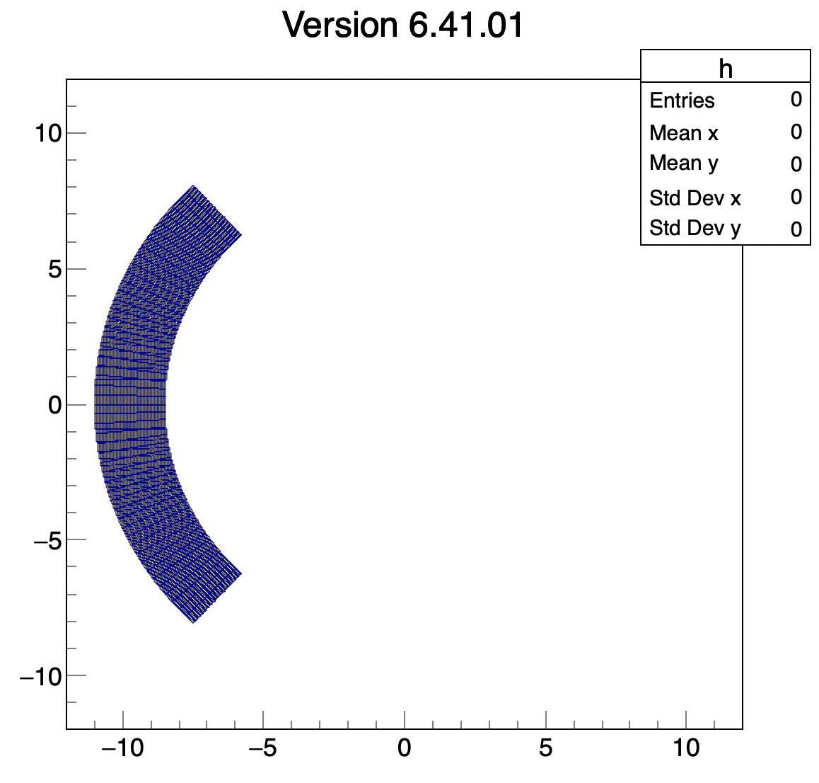
I see the same with ROOT master on Mac:

couet · July 22, 2026, 8:34am

The change of behavior has been introduced by this PR from @linev. You can see the explanations in the PR commit’s comments. @linev is on holidays right now. He can comment when he will be back.

atsushi · July 22, 2026, 9:57am

Thank you very much for the support.

I went through the source code committed there, trying to understand how it behaves.

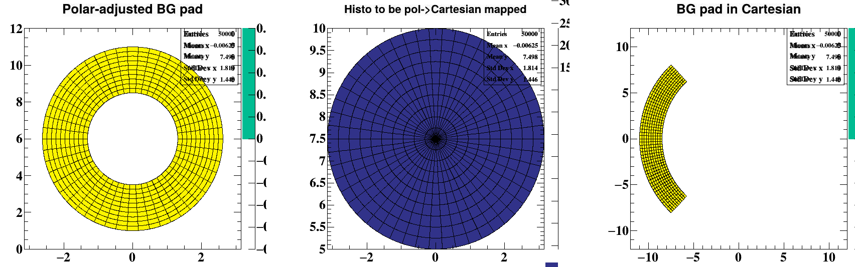
I ran the following test macro (v6.36) and got the attached plot:

{
   auto c1 = new TCanvas("c1", "Polar Histogram", 1200, 400);
   auto hBG = new TH2D("hBG", Form("Polar-adjusted BG pad"), 100,  -TMath::Pi(), TMath::Pi(), 100, 0, 12);
   auto h = new TH2D("h", Form("BG pad in Cartesian"), 100, -12, 12, 100, -12, 12);
   auto h2 = new TH2D("h2", "Histo to be pol->Cartesian mapped", 50, -1*TMath::Pi(), TMath::Pi(), 10, 5, 10);
   gRandom->SetSeed(10);
   for (int i = 0; i < 50000; i++) {
      double angle = gRandom->Uniform(-TMath::Pi(), TMath::Pi());
      double radius = gRandom->Uniform(5, 10);
      h2->Fill(angle, radius);
   }

   c1->Divide(3,1);
   c1->cd(1);
   hBG->Draw("");
   h2->Draw("SAME COLZ POL");
   cout << Form("Uxmin: %.2f, Uxmax: %.2f, Uymin: %.2f, Uymax: %.2f", gPad->GetUxmin(), gPad->GetUxmax(), gPad->GetUymin(), gPad->GetUymax()) << endl;
   c1->cd(2);
   h2->Draw("COLZ POL");
   c1->cd(3);
   h->Draw();
   h2->Draw("SAME COLZ POL");
}

My findings here are that the current “pol” option gives the actual polar coordinate of \theta = 2\pi \frac{x_{pol} - x_{BG}^{min}}{x_{BG}^{max} - x_{BG}^{min}} and r \propto y_{pol} - y_{BG}^{min} , where x,y_{BG}^{min,max} are the xy-range of the background histogram objects (hBG for 1st pad, h2 for 2nd pad, h for 3rd pad) and x,y_{pol} are the xy-value at each bin of the histogram objects drawn with “pol” option. For example, in the 3rd plot, the angle range is limited because calculating something like \theta = \frac{3.14 + 12}{24} for x=3.14 bin of h2 object.

Though the histogram itself in the first drawing is geometrically correct, the axis is taken from the background histogram object. Anyway, let’s wait for comments from the committer.

Atsushi

couet · July 22, 2026, 10:59am

Yes it is better @linev does the follow up.

linev · July 23, 2026, 8:01am

Hi Atsushi,

Yes, implementation of “POL” draw option was changed starting from ROOT 6.36.
Previous implementation had many problems and didn’t work correctly in many use-cases.
Just try to draw hpxpy histogram from hsimple.C example in polar coordinates. Especially interactive zooming was a real mess. Therefore I had doubts that such drawing can be used in productive work.

As you find out now polar coordinates recalculated from histogram X/Y ranges at the moment when painting performed. This let fix many existing problems but change produced plots. Main advantage of new approach - one do not need to create special axis histogram and can easily switch between different histogram draw options.

One can try to extend ROOT code and allow to use natural polar coordinates as histogram axes - but removing old problems. This can be done as “POLN” draw option. If you are interested - I can try to provide such option.

Regards,
Sergey

atsushi · July 23, 2026, 3:55pm

Dear Sergey

Thank you for the reply. I saw the motivation for the modification.

One can try to extend ROOT code and allow to use natural polar coordinates as histogram axes - but removing old problems. This can be done as “POLN” draw option. If you are interested - I can try to provide such option.

Yes, I would like to have such an option. With the current implementation, the lower and upper boundaries of the x-axis are bound to \theta = 0, 360^\circ, as far as I understand. However, in my use cases, I fill histograms with polar coordinate (e.g. describing hit maps on radially designed detectors) with the x-range of the histogram being [-\frac{1}{2}\pi, \frac{3}{2}\pi] for example, not always [0, 2\pi] . Therefore, I would like to request some tools to rotate the Cartesian-mapped histogram.

Thank you for the support,
Atsushi

linev · July 24, 2026, 3:16pm

Dear Atsushi,

I create PR which implements new “POLN” and “POLF” draw options.

github.com/root-project/root

[hist] implement new POLF and POLN draw options (#22913)

master ← linev:improve_hist_polar

opened 03:03PM - 24 Jul 26 UTC

linev

+96 -35

Since ROOT 6.36 implementation of "POL" draw option was changed. Angle and radi…us range automatically scaled to visible histogram range filling full 2*Pi angle and [0..max] radius range. This let display TH2 in polar coordinates for any provided range settings, but produced plots are not intuitive. Therefore two new options for polar coordinates were introduced. "POLF" - fixed polar coordinates. In such case full histogram X range mapped to -PI .. +Pi. And Y axis mapped to radius. In case of histogram zooming angle and radius of each bin remains the same (therefore name "fixed"), just number of displayed bins are reduced. "POLN" - natural polar coordinates. In this case X axis directly represents angle value in radians (therefore name "natural") and Y axis is just radius. Such functionality was requested in https://root-forum.cern.ch/t/64949/ Also "POL" was modified. Now X range mapped to [-180 .. 180) range making more intuitive presentation when central histogram X region displayed near angle 0 on the right side of polar plot.

Can you try it to check if it works as you expected.

Regards,
Sergey

atsushi · July 26, 2026, 10:08am

Dear Sergey,

Thank you for the update. I tried the new “POLN” option, but I am afraid that the mapping to the Cartesian coordinate is not rigid in some cases, even without zooming.

In the code below, I provide two typical cases (in the case switch part).

{
   Double_t rRange[2], xRange[2], yRange[2];
   Int_t caseID = 1;
   switch (caseID) {
   case 0:
      rRange[0] = 5;
      rRange[1] = 10;
      xRange[0] = -12;
      xRange[1] = 12;
      yRange[0] = -20;
      yRange[1] = 20;
      break;
   case 1:
      rRange[0] = 1;
      rRange[1] = 2;
      xRange[0] = -3;
      xRange[1] = 3;
      yRange[0] = -3;
      yRange[1] = 3;
      break;
   }

   TString polOpt = "POLN";
   auto c1 = new TCanvas("c1", "Polar Histogram", 600, 600);
   auto hBG = new TH2D("hBG", Form("Version %s, %s", gROOT->GetVersion(), polOpt.Data()), 100, xRange[0], xRange[1], 100, yRange[0], yRange[1]);
   auto hPol = new TH2D("hPol", "Polar Plot", 50, -0.5*TMath::Pi(), 1.5*TMath::Pi(), 50, rRange[0], rRange[1]);
   gRandom->SetSeed(10);
   for (int i = 0; i < 50000; i++) {
      double angle = gRandom->Uniform(-0.25*TMath::Pi(), 1.1*TMath::Pi());
      double radius = gRandom->Uniform(rRange[0], rRange[1]);
      hPol->Fill(angle, radius);
   }

   hBG->Draw("");
   hPol->Draw(Form("SAME COLZ %s", polOpt.Data()));
}

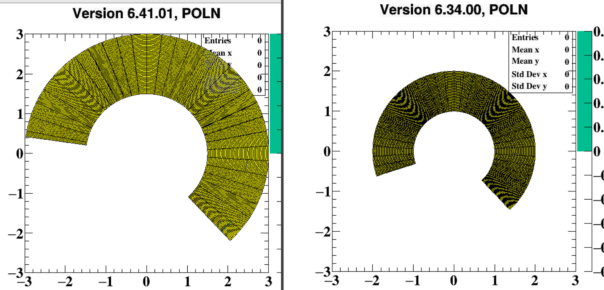
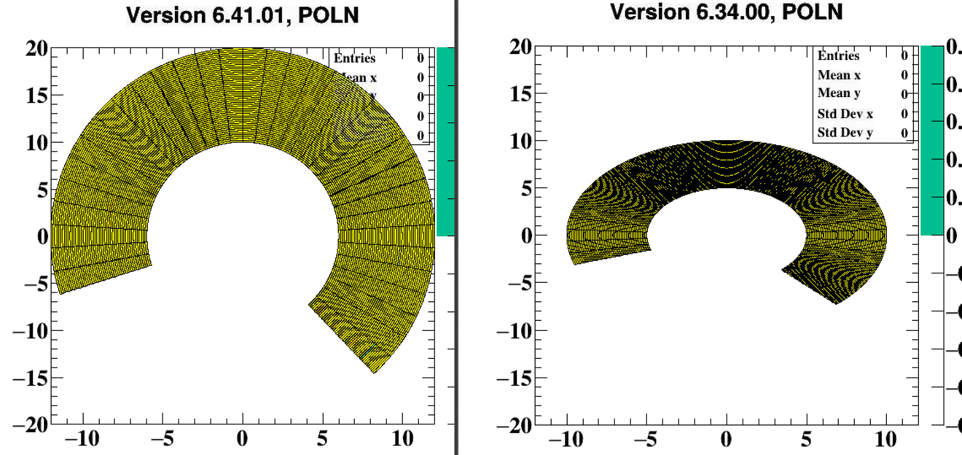
The attached plots show the result of this macro.

case = 0: Even though the radius range is smaller than the x and y-ranges of hBG, the “POLN” plots extend to the full range of hBG.
case = 1: When the x-range of hBG is smaller than \pi, the \theta range gets affected.

In both of these plots, i would expect to see plots that are produced by the 6.34 version, which perfectly matches the r\cos\theta, r\sin\theta to the hBG axes.

I believe that the consistency of the coordinate definition is essential when “POLN SAME” option is used, for example when radially designed detectors are overlaid with other detector components or tracks. May I ask you to design the “POLN” option accordingly?

Thank you,
Atsushi