Weird Plotting behavior with TGraph

[Mdrueke]

Hey guys,
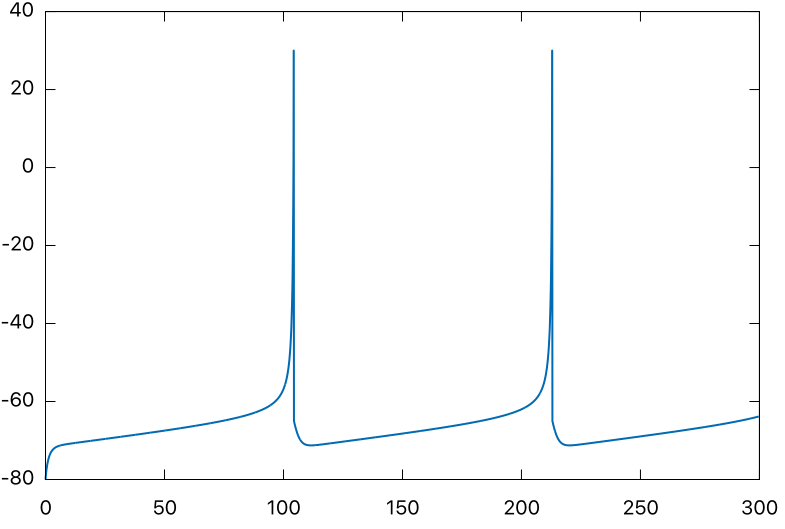
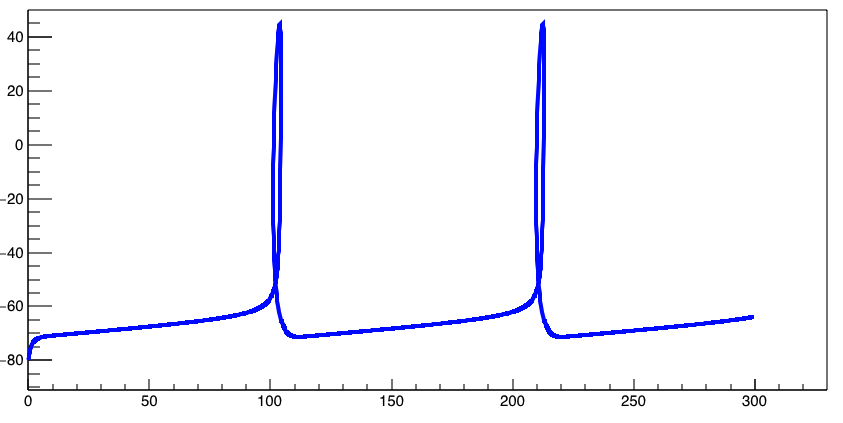
I’m new to ROOT (and programming). I implemented a model in C++ and would like to output the result with ROOT. The Plot looks fine when i use gnuplot, but weird if I use ROOT. It’s hard to explain, the ROOT plot somehow shows some kind of loops (which do not appear in gnuplot). I appended an image (and my Code).

#include <iostream>
#include <cmath>
#include <vector>
#include "TApplication.h"
#include "TCanvas.h"
#include "TGraph.h"


using std::cout;
using std::cin;
using std::endl;
using std::vector;

double a{0.1};
double b{0.26};
double c{-65};
double d{2};

double t_max{100};
double dt{0.1};
double v_0{-80};
double u_0{0};
double I{9.0};

struct timetrace{
    vector<double> t;
    vector<double> v;
    vector<double> u;
    float rate;
};

double dv(double v, double u, double I){
    return (0.04 * pow(v, 2.0) + 5 * v + 140 - u + I);
}

double du(double v, double u){
    return (a * (b * v - u));
}

timetrace V_t_trace(){
    int quantity{static_cast<int>(t_max/dt)-1};
    vector<double> t_array, v_array, u_array;
    t_array.reserve(quantity);
    v_array.reserve(quantity);
    u_array.reserve(quantity);
    //arrays that hold runge-kutta values:
    double u1,u2,u3,u4,v1,v2,v3,v4;
    timetrace trace;
    t_array.push_back(0);
    v_array.push_back(v_0);
    u_array.push_back(u_0);
    int spike_count{0};
    for(int i=1; i < quantity - 1; ++i){
        t_array.push_back(i * dt);
        /* EULER
         v_array.push_back(v_array[i-1] + dv(v_array[i-1], u_array[i-1], I) * dt);
         u_array.push_back(u_array[i-1] + du(v_array[i-1], u_array[i-1]) * dt);
         */
        
        // Runge-Kutta:
        u1 = du(v_array[i-1] , u_array[i-1]) * dt;
        v1 = dv(v_array[i-1] , u_array[i-1], I) * dt;
        u2 = du(v_array[i-1] + v1/2.0 , u_array[i-1] + u1/2.0) * dt;
        v2 = dv(v_array[i-1] + v1/2.0 , u_array[i-1] + u1/2.0, I) * dt;
        u3 = du(v_array[i-1] + v2/2.0 , u_array[i-1] + u2/2.0) * dt;
        v3 = dv(v_array[i-1] + v2/2.0 , u_array[i-1] + u2/2.0, I) * dt;
        //TODO: Check if this is correct!
        u4 = du(v_array[i-1] + v3 , u_array[i-1] + u3) * dt;
        v4 = dv(v_array[i-1] + v3 , u_array[i-1] + u3, I) * dt;
        u_array.push_back(u_array[i-1] + (u1+2.0*u2+u3+u4)/6.0);
        v_array.push_back(v_array[i-1] + (v1+2.0*v2+v3+v4)/6.0);
        // Reset condition:
        if (v_array[i] >= 30){
            spike_count++;
            v_array[i-1] = 30;
            v_array[i] = c;
            u_array[i] += d;
        }
    }
    trace.rate = spike_count/t_max * 1000;
    trace.t = t_array;
    trace.v = v_array;
    trace.u = u_array;
    return trace;
}


int main(int argc, const char * argv[]) {
    //request values
    cout << "a = ";
    cin >> a;
    cout << "b = ";
    cin >> b;
    cout << "c = ";
    cin >> c;
    cout << "d = ";
    cin >> d;
    cout << "Input current = ";
    cin >> I;
    cout << "t_max = ";
    cin >> t_max;

    timetrace voltage_trace = V_t_trace();
    vector<double> t = voltage_trace.t;
    vector<double> v = voltage_trace.v;
    vector<double> u = voltage_trace.u;
    float rate = voltage_trace.rate;
    cout << "Firing rate is " << rate << " Hz\n";
    

    
    //Plotting
    TApplication* myApp = new TApplication("myApp", 0, 0) ;
    
    TCanvas *c1 = new TCanvas("c1","Izhikevich model",200,10,1000,500);
    TGraph* gr = new TGraph(v.size(),&t[0],&v[0]);
    gr->SetLineColor(kBlue);
    gr->SetLineWidth(4);
    gr->SetMaximum(50.);
    gr->Draw("AC");
    c1 -> Update();

    // Run the TApplication to produce all of the plots
    myApp->Run() ;
    return 0;
}

[Wile_E_Coyote]

    gr->Draw("AL");

[Mdrueke]

This is the gnuplot output: