Now I am getting a minor issue in UL calculation with this. With observed event = 0, expected background = 0.4, relative uncertainty on background = 0.71, I estimate the UL by using StandardHypoTestInvDemo.C macro and the CountingModel.C macro(which is already given in this question).
With 90% CL the upper limit on signal yield found to be 1.22 ± 0.07 when I use the code as StandardHypoTestInvDemo(“CountingModel.root”,“w”,“ModelConfig”,"",“data”,0,2,false,30,0,8,1000,true);
But if I decrease the maximum value of the parameter to 5, and use the same as StandardHypoTestInvDemo(“CountingModel.root”,“w”,“ModelConfig”,"",“data”,0,2,false,30,0,5,1000,true); the UL changes slightly and becomes 1.09 ± 0.066 at 90% CL.
Here my question is why the UL changes from 1.22 to 1.09 when I decrease the maximum value of the parameter. Also how to decide what maximum value of the parameter to be used. If I change the maximum value to 10 similarly the UL also changes. Can you please let me know?
The difference is probably explained by the fact you scan in different points. Try to scan on the same points (e.g. 20 points between [0,5] and 32 points between [0,8].
Also , since you are using toys , you might want to increase their number to get a more stable result.
Thank You so much! If I increase the number of toys I am getting a stable result.
For
observed events (nobs) = 1, expected background (b) = 1.30, relative uncertainty (sigma b ) = 0.354,
Earlier I was using the uncertainty as Gaussian.
Now I want to use the uncertainty as Poisson. Can you please have a look at the modified model that I am using now? Now If I vary the uncertainty (sigma b) to 0.7, there seems to be no change in the Upperlimit. I am using for 90% UL. Is it there any problem with the modified model now?
In both the Poisson uncertainty case, I am getting same UL= 2.97.
used as:
StandardHypoTestInvDemo(“CountingModel_poisson_new.root”,“w”,“ModelConfig”,"",“data”,0,2,false,30,0,10,1000,true);
Also another thing, is it good to cite Feldman Cousins original paper PRD V57 #7, p3873-3889 for this method? In the original paper the uncertainty on the background is not considered. Or one can cite as modified Feldman Cousins method and give the link of https://root.cern.ch/doc/v608/StandardHypoTestInvDemo_8C.html macro.
Also in this method, the statistical and the systematic uncertainty on the background are added in quadrature to get a total uncertainty on the background in the model, is it correct?
If you use a Poisson constraint , sigmab is not anymore a parameter of the model. The Poisson needs only one parameter, b and therefore its standard deviation (i.e. sigma) will be sqrt(b).
If you are using the double side test statistics and CL(S+B), not CLs, you should cite the Feldman COusins papers and you could cite the RooStats paper (https://arxiv.org/abs/1009.1003) and the link to the macro for the procedure
Thank You so much for giving this information!
Sorry to bother you again.
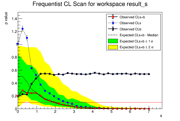
For no. of observed event = 0, number of expected background events = 0.4 and relative uncertainty = 0.7, Following scan plot is obtained from the same counting model as previously(Posisson model with a Gaussian constraint):
If possible for you can you please explain why the blue dot curve (CLs curve) goes beyond 1 as S->0 (as you can see it is going upto1.25)? I think it should be less than 1 (sorry if I am wrong)?
Also just for clear clarification, based on what values the expected median
and ±1/2sigma bands are calculated?
I will really appreciate your help if you can give a quick response.
Yes it is correct, for studying upper limits where you don’t have real signal in the data you are looking at, CL(S+b) should be smaller than CL(b) and therefore CL(s) < 1. So probably what is happened is a problem with the toys or fitting these toys that are used for computing the upper limit. I would ignore these cases and perform the scan only in the region where s> 1.
Expected mean is obtained using the median test statistic distribution for B only toys (the one used for computing CL(B)) and use that value as it would be the observed value of the test statistics.
In the same way the 0.16 and (1-0.16) quantiles of the B test statistic distributions are used for the expected 1 sigma and the 0.025 and 0.975 quantiles for the 2 sigma bands
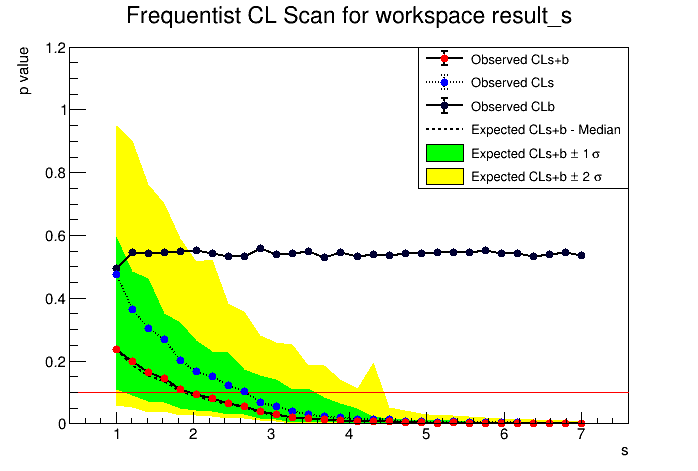
Now I do the scan for s(1,7). The following scan plot is obtained.
Following result is obtained:
The computed upper limit is: 1.94846 +/- 0.0319551
Expected upper limits, using the B (alternate) model :
expected limit (median) 1.87559
expected limit (-1 sig) 1.11374
expected limit (+1 sig) 3.57288
expected limit (-2 sig) 1.17407e-16
expected limit (+2 sig) 4.44757
The CL(s+b) UL now becomes 1.94. Whereas with s(0,7) it was 1.98. There is no big change:)
I think it is correct now. Can you please let me know how to decrease the bump of +2sigma plot (yellow) around S= 4.3.
I used the code as StandardHypoTestInvDemo(“fc_counting_model.root”,“w”,“ModelConfig”,"",“data”,0,2,false,30,1,7,10000,true); for FC limit.
I think you have explained the expected mean and band calculation procedure for CL(s+b) method. Can you give me any references so that I can gain more understandings?
You can try increasing the toys statistics, both for S+B and B toys to see if bump goes away, otherwise it is possible that is due to the discreteness of the Poisson distributions.
For the references I would need to look if I find a paper or presentations explaining the method in more details
Thank You! Yes, the bump vanishes with increasing the no. of TOY.
I have another query that I use the code CountigModel.C.
Where the inputs are nobs, b and sigmab.
sigmab is the relative uncertainty in b.
The uncertainty include both statistical and systematic uncertainty on b (added in quadrature) .
Here my doubt is that shall I consider only the systematic uncertainty to get the relative uncertainty for the model?
Or is it fine to add both statistical and systematic uncertainty for considering the Gaussian constraint?
Because the model is constructed as
w.factory(“Poisson:pdf(nobs[0,15],nexp)”);
w.factory(“Gaussian:constraint(b0[0,10],b,sigmab[1])”);
w.factory(“PROD:model(pdf,constraint)”);
Here my doubt is that the poisson pdf already contains the statistical uncertainty and the Gaussian uncertainty should be only systematic uncertainty? Otherwise how to include the statistical uncertainty in the background into the model?
I am sorry that It is not clear in the twiki tutorial link. I think the doubt is clear to you. Otherwise please let me know.
Another thing also what is being fitted in this method to get the UL calculation. Is it the toy data set generated by the model (Poisson*Gaussian model)? I will really appreciate again your help if you could clarify my doubts.
sigmab should contain all the uncertainties you have before (e…g from previous measurements or other estimation) on b. It is a question of definition on how you call these uncertainties.
Fluctuation of b due to current the data (nobs) are already considered.
Thank you so much for the clarification.
So as I understand so far in this method a model is created with observed events, expected background and the uncertainty on the background(all types statistical and systematics).
Then a hypothetical data set is generated by the model.
Here we want to disprove the null hypothesis is the S+B model, while the alternate hypothesis is the B only model.
Then Frequentist calculator is configured with double sided profile likelihood test statistics for FC method and number of toys.
But how the fitting to toy generated data set playing a role here? Can you please clarify this. Also is fitting is done by the same model that we use for creating toy data?
I find some difference in the case of CL_{s+b}(FC), CL_{s}, and asymptotic CL_{s} method of obtaining UL for the following case.
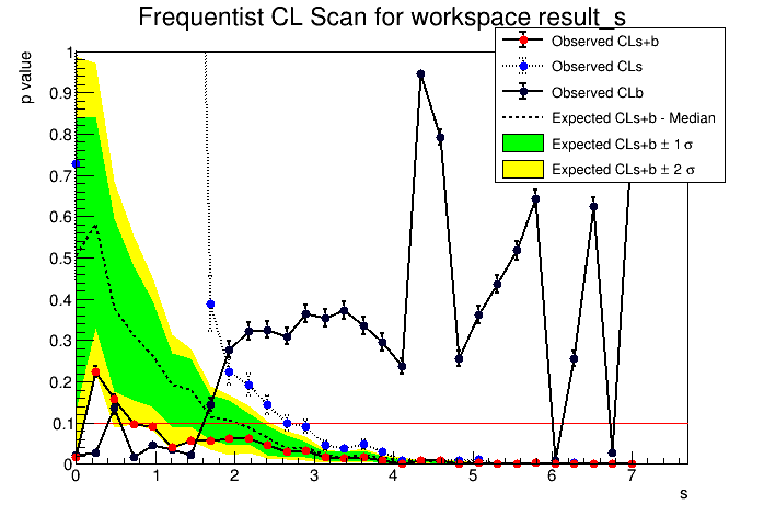
Now I am trying to obtain the 90% UL in the case of the number of observed events = 0, number of expected background =0 and with a small uncertainty = 0.036
With the CL_{s+b} (FC) method the obtained UL = 0.7 at 90% CL. The program is used as
StandardHypoTestInvDemo(“CountingModel_zerobkg_zeroobs.root”,“w”,“ModelConfig”,"",“data”,0,2,false,30,0,7,1000,true); The corresponding scan plots is shown here.
But if I use directly Feldman-Cousins paper with observed event = 0 and expected background = 0 then the 90% CL upper limit on signal yield = 2.44.
With CL_{s} method, UL = 2.43 at 90% CL
with asymptotic CL_{s}, UL = 1.36
(for all three case same attached model is usedCountingModel_zerobkg.C (1.6 KB) )
Can you please let me know how to bring a UL close to 2.4 in the case of CL_{s+b} (FC) method? Again I will really appreciate your help.
What you are seeing is due to the discreteness of the Poisson distribution. If you have zero systematics, you will get the same values as in the FeldmanCousins paper (2.44), but by adding a small systematic, the test statistics distributions get a small smearing and the result is a lower upper limit.
You can try reducing further the systematic (e.g. sigmab=0.001) and you will get a result close to the 2.44 value obtained when the systematics are zero
Sorry, I am again. Can you please clarify the following queries.
I was comparing the CL_{s+b} UL, for nbkg =0 and nobs =0,1,2 and 3 for a small uncertainty of 0.04 with that obtained from original FC paper.
(1) (Usually(naturally/naively), the inclusion of uncertainties would move UL to a lager value than that without uncertainties. but why am I getting a smaller values?
(2) Even I tried to set the uncertainty =0 and with the model, I tried to estimate the UL. But in this case also the UL becomes small as compare to FC paper. Actually if uncertainty is set to zero then the UL obtained from CL_{s+b} method should match to that values obtained from FC original paper?
CountingModel_zerobkg_zerouncern.C is with uncetainty =0(where I have modified) and CountingModel_zerobkg.C with small uncertainty. Can you also please check both the models. If they are correctly modeled.
Also, I tried with non zero nbkg, e.g nbkg = 0.51 and nobs =1 with relative uncertainty = 0.35, the UL = 3.2; whereas that from FC original paper UL is in the range of 3.86-3.36. So is there any problem with CL_{s+b} method I am getting smaller value although the expectation is larger?
I hope that you have understood my last concerns. Please let me know if it’s unclear.
Actually, for setting UL by FC method with uncertainty, a POLE (See http://www3.tsl.uu.se/∼conrad/pole.html, J. Conrad et al., Phys. Rev. D
67, 012002 (2003)) program is being used in our collaboration. While for the first time, I used CL_{s+b} method in our collaboration by contacting here. For which, there are many questions that arose to test properly this method with different situations. So in this process, I asked here which I couldn’t solve myself.
Hi,
Thank you for this useful investigation and for the link of the program of J…Conrad.I will look into it and verify your results. As I said, it is expected that introducing a small systematic uncertainty improves the limit, and this is due to the discreteness of the Poisson distribution.
Once you introduce some systematics, your test statistics distribution is not anymore discrete, you can see in the plots and this will give you a better limit, while before the limit was worse but with some overcoverage.
Yes, I am getting better limits (small numbers) with CL_{s+b} method after adding uncertainties.
But it is expected that the UL will become worse (higher number) after adding uncertainties as you may find from some statistical papers like Cousins-Highland paper.
I am just a beginner at this type of statistics calculations. But according to my understanding, at the end of the day, all methods should give similar results (either all method should give better or worse limits). Maybe the numbers vary slightly.
I am a new student not familiar with statistics…But i need a help…I need to get an upper limit on my signal.
Say i have a signal “s” and a background “b” with some error(both statistical and sytematic). Note that “s” and “b” are actually slopes obtained after fitting experimental data points. Now i want to quote an upper limit on fraction of signal i.e on variable ((s-b)/s) with a certain confidence level. Please also note that this fraction of signal needs to physically between 0-1 but experiementally i am do getting -ve values and values >1.
By surfing through net i came across your thread. Could you please help me how to do this…?
But in your case you have determined “s” and “b” from fitting. You want to put a limit on ((s-b)/s). I guess you need to change the model accordingly or your case follows a completely different procedure.
I am also a student and not an expert on limit setting procedures. May be someone from root may help you.