Hi,
I went through the current TProfile::Chi2Test() implementation and the underlying TH1::Chi2Test(..., "WW") code path. The scale invariance is not a numerical accident: it follows directly from the statistical hypothesis implemented by the weighted-histogram test.
For two profiles, let
m_{1i},\;m_{2i}
be the bin means returned by the profiles, and let
e_{1i},\;e_{2i}
be the corresponding standard errors of the mean.
TProfile::Chi2Test() currently forces the comparison of two TProfile objects through
TH1::Chi2Test(..., "WW")
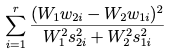
and the weighted-weighted test uses, bin by bin,
\chi^2_{\mathrm{WW}}
=
\sum_i
\frac{
\left(
S_1m_{2i}-S_2m_{1i}
\right)^2
}{
S_1^2e_{2i}^2
+
S_2^2e_{1i}^2
},
where
S_1=\sum_i m_{1i},
\qquad
S_2=\sum_i m_{2i}.
Define
r=\frac{S_2}{S_1}.
Then the same statistic can be written as
\boxed{
\chi^2_{\mathrm{WW}}
=
\sum_i
\frac{
\left(
m_{2i}-r\,m_{1i}
\right)^2
}{
e_{2i}^2+r^2e_{1i}^2
}
}.
This makes the source of the scale invariance explicit.
If the second profile is a global rescaling of the first,
m_{2i}=c\,m_{1i},
with correspondingly scaled errors
e_{2i}=|c|e_{1i},
then
S_2=cS_1
and therefore
r=c.
Hence every numerator vanishes:
m_{2i}-r\,m_{1i}
=
c\,m_{1i}-c\,m_{1i}
=
0,
so that
\boxed{
\chi^2_{\mathrm{WW}}=0
}
for any non-zero global scale factor c.
So the present TProfile::Chi2Test() is not testing
H_0:\quad \mu_{1i}=\mu_{2i}
bin by bin.
It is effectively testing a different hypothesis:
H_0:\quad
\mu_{2i}=c\,\mu_{1i}
for an overall normalization factor.
That hypothesis makes sense for a histogram homogeneity test, where one often wants to compare shapes independently of the total normalization, but it is not the usual equality test for profile means.
For two independent profiles, the natural profile-to-profile test is instead based directly on the difference of the estimated means:
\Delta_i=m_{1i}-m_{2i}.
Under
H_0:\quad \mu_{1i}=\mu_{2i},
and assuming independent profile estimates,
\operatorname{Var}(\Delta_i)
=
e_{1i}^2+e_{2i}^2.
Therefore the standardized residual is
r_i
=
\frac{
m_{1i}-m_{2i}
}{
\sqrt{e_{1i}^2+e_{2i}^2}
},
and the corresponding chi-square statistic is
\boxed{
\chi^2_{\mathrm{profile}}
=
\sum_i
\frac{
\left(
m_{1i}-m_{2i}
\right)^2
}{
e_{1i}^2+e_{2i}^2
}
}.
For independent approximately Gaussian bin-mean estimates, this is the direct test of profile equality.
If k valid bins are compared and no additional common parameter is fitted, the natural number of degrees of freedom is
\boxed{\mathrm{ndf}=k},
not k-1.
The loss of one degree of freedom in the weighted-histogram homogeneity test comes from the normalization constraint. That constraint is not part of the ordinary equality-of-profile-means problem.
For the example
m_1=(10,20,30),
m_2=(20,40,60),
with
e_1=(0.1,0.1,0.1),
and
e_2=(0.2,0.2,0.2),
the current weighted-histogram path gives
\chi^2_{\mathrm{WW}}=0,
because the second profile is exactly twice the first.
But the direct profile-equality statistic gives
\chi^2_{\mathrm{profile}}
=
\frac{(10-20)^2}{0.1^2+0.2^2}
+
\frac{(20-40)^2}{0.1^2+0.2^2}
+
\frac{(30-60)^2}{0.1^2+0.2^2}.
Since
0.1^2+0.2^2=0.05,
this becomes
\chi^2_{\mathrm{profile}}
=
\frac{100+400+900}{0.05}
=
\boxed{28000},
with
\boxed{\mathrm{ndf}=3}.
So the two procedures are answering fundamentally different statistical questions.
There are also two additional consequences of reusing TH1::Chi2Test("WW") for profiles.
First, the histogram code treats
\sum_i m_i=0
as an empty histogram condition.
For a TProfile, however, a profile such as
(-1,+1)
can be perfectly well populated and have finite uncertainties, while its bin means sum to zero. A zero sum of profile means is therefore not an emptiness criterion.
Second, the weighted-histogram implementation reduces the degrees of freedom when both bin contents are zero. For a profile,
m_{1i}=m_{2i}=0
does not imply that the bin contains no observations. Both profiles may contain many entries whose estimated means happen to be zero.
So the mismatch is not limited to scale invariance; it comes from applying histogram-content semantics to quantities that, in a TProfile, represent estimated conditional means.
A cleaner implementation would therefore separate the two use cases.
For TProfile versus TProfile, the default equality test could use
\chi^2
=
\sum_i
\frac{
(m_{1i}-m_{2i})^2
}{
e_{1i}^2+e_{2i}^2
},
with bins included according to the validity of their profile estimates rather than according to histogram-count semantics.
More generally, if full covariance information is available, the same test is
\boxed{
\chi^2
=
\Delta^{T}
C_{\Delta}^{-1}
\Delta
},
with
\Delta
=
m_1-m_2.
For independent profiles,
C_{\Delta}
=
C_1+C_2.
If the two profiles are built from correlated samples, then the cross-covariance terms must also be included:
C_{\Delta}
=
C_1+C_2-C_{12}-C_{21}.
An explicitly named shape-only or scale-free comparison could still use a normalization-fitted statistic if that is desired, but it should be distinguished from the default test of equality of profile means.
So the observed scale invariance is mathematically consistent with the current "WW" implementation, but it also shows that the current TProfile::Chi2Test() is testing a different null hypothesis from the one a user would normally expect when comparing two profiles.