Signal strength in extended maximum likelihood method

Dear @moneta, Dear all,

I used the Extended maximum likelihood method (or profile likelihood) with Gaussian for a signal and first-order polynomial for a background, to put an upper limit on cosmogenic peaks in my data. Here is my code if you are wondering how I did it. Everything worked fine and I have now my upper limits as well.

But there is one thing that I don’t understand and want to clear it up. I defined ‘Nsig’ and ‘Nbkg’ as a number of signal/bkg events in a particular range but I saw in my collaboration that people have defined their signal and background like this.

Of course, their case signal represents half-life and they put a limit on that. But I am wondering how would i define ‘Nsig’ and ‘Nbkg’ in my case because i didn’t define Nsig with a formula like this. Except that, i am using the same approach as they are. I would really appreciate if you help me understand this concept.

Thank you in advance!

Maybe @jonas can help

Hi @cosmogenic!

I don’t quite understand your concern. You said that you “defined ‘Nsig’ and ‘Nbkg’ as a number of signal/bkg events in a particular range”, and that’s exactly how in the paper you quoted it is used too. Only that they call it \mu^S and \mu^B, and the width of the range is called \Delta E.

And the RooAddPdf does exactly what happens in equation (3): the normalized sum of two PDFs.

I hope this makes things clearer, and if they are not, please explain your question in more detail so I can give the suitable answer.

Cheers,
Jonas

Hi @jonas,

Thanks for your reply. This is what i wanted to know if μ^s and μ^B are the same as mine Nsig and Nbkg. Because i define Gaussian distribution for the signal and polynomial distribution for a background in the range (1223 - 1323) and then I am defining RooRealVar Nsig(“Nsig”, “Nsig”,10000,0,10000), like this. Is this automatically in terms of the equation looks like μ^s as in the paper?

Do you understand what i am saying? If not please let me know. And i am sorry if i am asking stupid questions.

Yes, exactly, your Nsig and Nbkg are used just like \mu^S and \mu^B in the paper!

Only a little unrelated note, setting the parameters values and ranges like this is not a very good idea:

RooRealVar Nsig(“Nsig”, “Nsig”,10000,0,10000)

The initial parameter value, 10000, is equal to the maximum allowed value. This would be a problem for fitting, because the minimizer doesn’t like it if a parameter value is at the boundary. You should extend your boundaries a bit, maybe by a factor 10.

Cheers,
Jonas

Dear @jonas,

Thanks for your reply. To explain you, what I really wanted to understand, fortunately, I found one post on root forum. In this post RooStats: Change of Constraint does not change Profile Likelihood Plot, they are doing the same statistical analysis as mentioned in the paper above.

In this post, you can see that they are explaining μ^s by using a variables of half live, lifetime of experiment and conv_factor as defined in paper and then they are using these parameters in “nsig”. I have put this screenshot below.

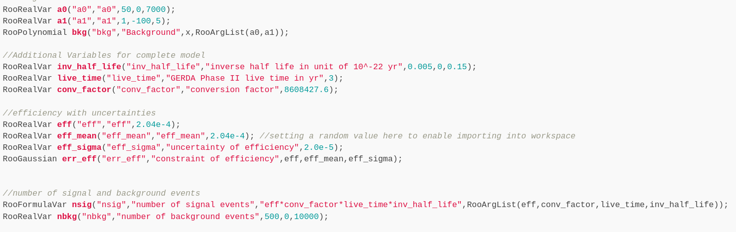
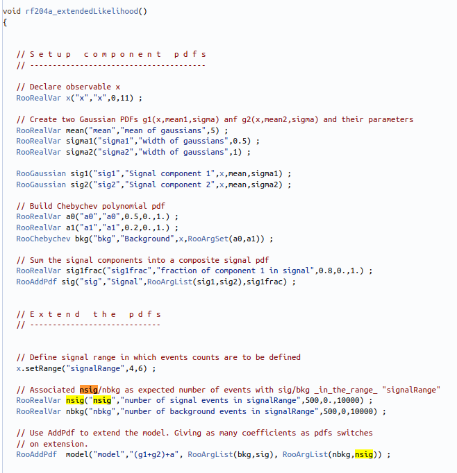
But in my case, if you see my code in the first post, i am using “Nsig” and “Nbkg” as the expected number of events in the signal and background region, right?

More or less like here:

So, can you tell me which one for my case is relevant?

Thanks!

Dear @jonas,

Please let me know what do you think, if you have time. I would really appreciate it.

Thank you!

This topic was automatically closed 14 days after the last reply. New replies are no longer allowed.