You can “fix” whatever parameter you want.
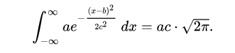
BTW. Note that the “area” parameter of a “gausn” is always its “full” integral. You integrate the function from some “xmin” to some “xmax”, so such “integral” will always be <= “area”.
You can “fix” whatever parameter you want.
BTW. Note that the “area” parameter of a “gausn” is always its “full” integral. You integrate the function from some “xmin” to some “xmax”, so such “integral” will always be <= “area”.
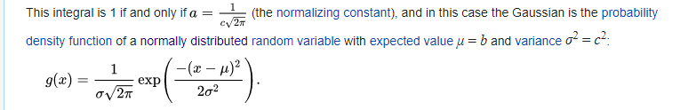
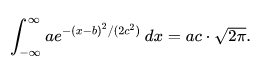
When you say full integral, it is the value of this first part below: 1/sigma*squareRoot(2Pi) .
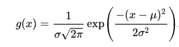
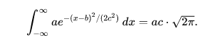
The integral, however , is the value below.
A bit confusing. When we fit gausn instead of gaus, do we tell somewhere in the code before it prints out the information, show the area as the 1st parameter. Obviously, the area is NOT equal to normalizating constant.
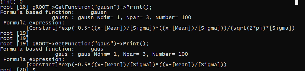
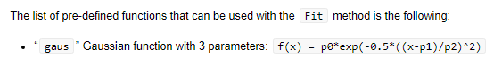
gROOT->GetFunction("gaus")->Print();
gROOT->GetFunction("gausn")->Print();
It’s nice that I can see quicker like that instead of going through the ROOT website. I wasn’t aware. Thanks for that.
That’s the website version.
![]()
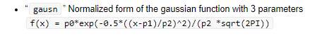
To be normalized to 1, p0 here should be set to squareRoot(2xPi )x sigma in gaus.
Gausn is actually different than PDF of the Gaussian function as said on this website.
Ok. let me try my shot to explain my confusion.
In gaus, we give height as parameter, it draws the shape nicely. In gausn, we need to give area to be drawn. By looking at the histogram, I can easily give the hight but not the area. I need to calculate the area from height x sigma x sqrt(2 x Pi) . Isn’t it tiring?
Yeah, I am aware of that.
Here below, how p0 parameter turns to an area as a fit parameter after fitting?
@Wile_E_Coyote
From terminal results, if I do gross area - background area with a calculator, it doesn’t match the ROOT net area result.
Is that normal!
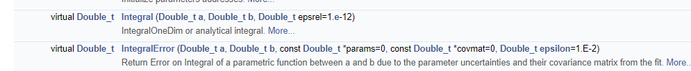
Try:
{
  TF1 *f = (TF1*)gROOT->GetFunction("gausn");
  Double_t area = 100., mean = 0., sigma = 1.;
  f->SetParameters(area, mean, sigma);
  std::cout << "area = " << area << std::endl;
  for (Int_t i = 1; i < 10; i++)
    std::cout << i << " : " << area - f->Integral(mean - i * sigma, mean + i * sigma) << std::endl;
}
BTW. Make sure that you use:
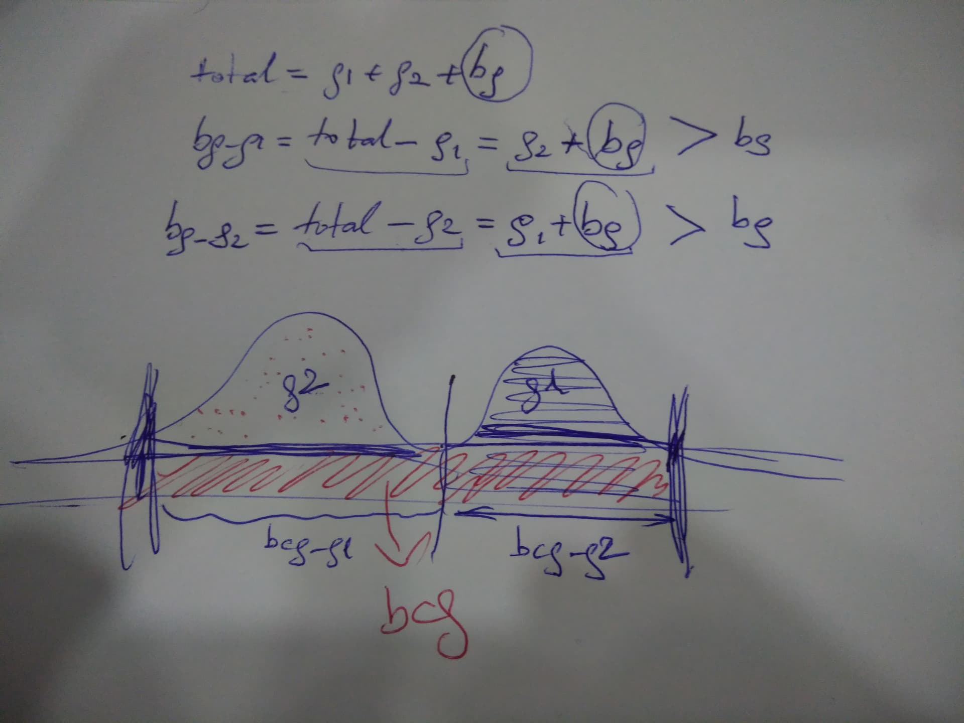
total = g1 + g2 + bg
bg_g1 = total - g1 = g2 + bg (i.e., it’s always >= bg)
bg_g2 = total - g2 = g1 + bg (i.e., it’s always >= bg)
{
TCanvas *c1 = new TCanvas("c1", "c1", 800,400);
c1->Divide(2,1);
c1->cd(1);
TF1 *f = (TF1*)gROOT->GetFunction("gausn");
Double_t area1 = 100., mean1 = 0., sigma1 = 1.;
f->SetParameters(area1, mean1, sigma1);
f->Draw();
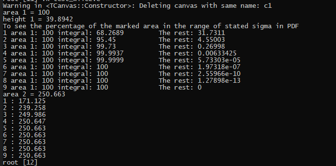
std::cout << "area 1 = " << area1 << std::endl;
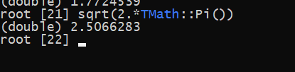
std::cout << "height 1 = " << area1/ (sigma1*sqrt(2.*TMath::Pi()) ) << std::endl;
Int_t i;
cout << "To see the percentage of the marked area in the range of stated sigma in PDF" << endl;
for (i = 1; i < 10; i++)
std::cout << i << " area 1: "<< area1 << " integral: " << f->Integral(mean1 - i * sigma1, mean1 + i * sigma1) << "\t\tThe rest: " << area1- f->Integral(mean1 - i * sigma1, mean1 + i * sigma1) << std::endl;
c1->cd(2);
TF1 *f2 = (TF1*)gROOT->GetFunction("gaus");
Double_t height2 = 100., mean2 = 0., sigma2 = 1.;
f2->SetParameters(height2, mean2, sigma2);
f2->Draw();
std::cout << "area 2 = " << sqrt(2.*TMath::Pi()) *height*sigma2 << std::endl;
for ( i = 1; i < 10; i++)
std::cout << i << " : " << f2->Integral(mean2 - i * sigma2, mean2 + i * sigma2) << std::endl;
}
I added more on that teaching code. What was your point about gausn?
BTW, I am suprised about the gaus plot above. Its x axis range is between + sigma and - sigma when we do not state it explicitly. Anyways.
That’s interesting because I wasn’t imagining the ROOT is calculating it like that. Surely, this calculation should be only valid for common (linked) background line, not for the separate bcg line approach. Right! I guess it won’t be valid if the peaks are way apart from each other, then in this case, we need to define 2 bcg functions. I guess ROOT regards the broken line as continous as if there was 1 line.
Question: When we say g1, don’t we mean the net area + its background ?
Answer: Ohh. NO, it’S not because we use the integral of g1 when we get the NET area of g1.
Namely, g1 and g2 are our NET sginals. ![]()
That’ amazing to see how easily the ROOT finds the net area.
I made it clear below with my worst drawing.
That’ why we limit ourselves within the g1 limits when we try to retrieve the bcg_g1.
For instance: we use lower and upper bin edges as limits.
double bcg_g1 = bcg->Integral(g1_X_LBE, g1_X_UBE) / BinWidth ;
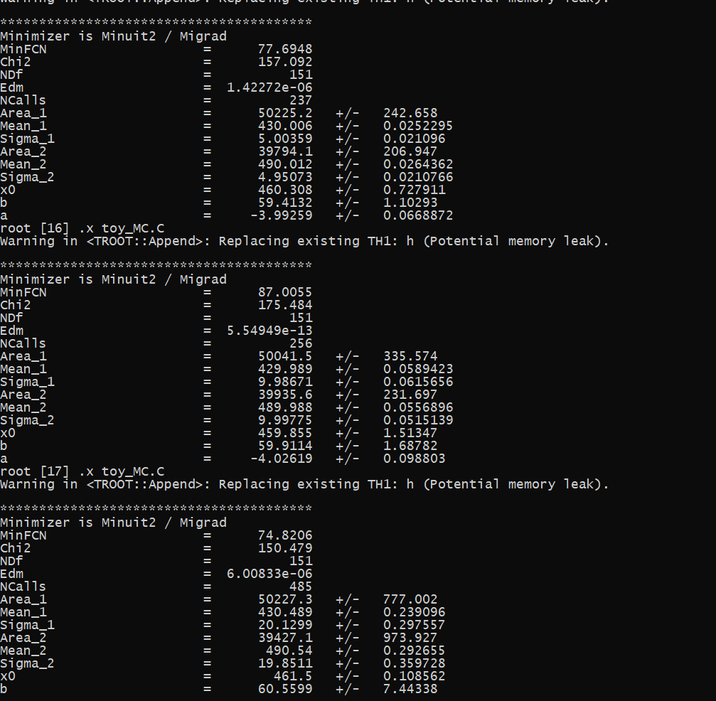
The “toy MC” (by default) sets the “sigma” parameter = 10 for both “gausn” peaks. Try to play with “sigma” = 5 and then with “sigma” = 20 (for both peaks, of course).
My little adapted code above, says nothing changes.
I mean I knew that after around 5 sigma, the integral percentage reaches to 100 percent already, so no need to go to infinity to retrieve the whole integral.
Is that your point?
For each “sigma” setting, you can play your games with “Integral” (comparing your “gross area”, “background area” and “net area”).
Ref: Gilmore’S fantastic book.
One question: What’s the differerence between the area found from gausn parameter and the integral value of g1 within the specified X-axis range?
I think evertime we limit ourselves within smaller x axis range than -+3sigma, our results from gausn parameter will always be (perceptively) bigger than the area from integral within the specified range.
Supportive info:
The area found from the gausn parameter = height x sigma x sqrt(2*pi) originally in the integral range of - infinity to + infinity.
On the other hand, the area found from specified gausn X range =
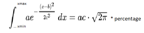
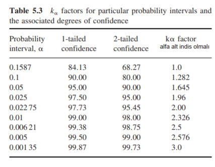
As we knew in advance and as we tested before, the X axis range becomes important if you choose the range smaller than -+5sigma which correspond to %99.9 . After even -+3sigma, x axis the coverage range becomes irrelavant due to %99 coverage.
Am I right in my arguments?
Obviously, the first parameter of the “gausn” function is by definition equal to the “a*c*sqrt(2*pi)” from your analytical formula.
What you said is correct Not just for Me, but for everbody.
My point was that we should always add this percentage (or you can call it as CORRECTION FACTOR) if you limit your range of interest (ROI) narrow in the case of , for instance, existing neighbouring peaks.
That’s all.