Problem in smearing histogram

Hi,

I use the following code to smear a histogram in two ways:

  1. Using the gRandom->Gaus(x,3.5)
  2. using x_res = x + 3.5 * TMath::Sqrt2() * TMath::ErfInverse(2. * rndm() - 1.)

the follwoing is my code :

{
gStyle->SetOptStat(2211);
gStyle->SetOptFit(1111);

TCanvas *c1 = new TCanvas("c1","Without constraint",800,600);
c1->Clear();
c1->Divide(2,2);

  auto h1=new TH1D("h1_gaus",
           "Mass (amu);Counts",
           101.0,39.5,140.5);

TH1D*h2 = new TH1D("h2","h2_Mass_resolution",101.0,39.5,140.5);
TH1D*h3 = new TH1D("h3","h3_Mass_resolution",101.0,39.5,140.5);


h2->SetLineColor(6);
  ifstream inp; double x;
  inp.open("try.txt");
  for (int i=1; i<=100; i++) {
    inp >> x;
    h1->SetBinContent(i,x);
    h2->SetBinContent(i, gRandom->Gaus(x,3.5));
    h3->SetBinContent(i, x + 3.5 * TMath::Sqrt2() * TMath::ErfInverse(2. * rndm() - 1.) );
  }

c1->cd(1);
h1->Fit("gaus","","",44.5, 130.5);
h1->Draw();
c1->cd(2);
h2->Fit("gaus","","",44.5, 130.5);
h2->Draw("");
c1->cd(3);
h1->Draw();
h2->Draw("HIST SAMES");
c1->cd(4);
h3->Draw("");
gStyle->SetOptStat(111111111);
c1->Update();

}

but when I run it I get the attached error :

How to resolve this ?

{
   gStyle->SetOptStat(2211);
   gStyle->SetOptFit(1111);

   auto c1 = new TCanvas("c1","Without constraint",800,600);
   c1->Divide(2,2);

   auto h1 = new TH1D("h1_gaus","Mass (amu);Counts",101.0,39.5,140.5);
   auto h2 = new TH1D("h2","h2_Mass_resolution",101.0,39.5,140.5);
   auto h3 = new TH1D("h3","h3_Mass_resolution",101.0,39.5,140.5);


   h2->SetLineColor(6);
   ifstream inp; double x;
   inp.open("try.txt");
   for (int i=1; i<=100; i++) {
      inp >> x;
      h1->SetBinContent(i,x);
      h2->SetBinContent(i, gRandom->Gaus(x,3.5));
//      h3->SetBinContent(i, x + 3.5 * TMath::Sqrt(2) * TMath::ErfInverse(2. * rndm() - 1.) );
      h3->SetBinContent(i, x + 3.5 * TMath::Sqrt(2) * TMath::ErfInverse(2.));
   }

   c1->cd(1);
   h1->Fit("gaus","","",44.5, 130.5);
   h1->Draw();

   c1->cd(2);
   h2->Fit("gaus","","",44.5, 130.5);
   h2->Draw("");

   c1->cd(3);
   h1->Draw();
   h2->Draw("HIST SAMES");

   c1->cd(4);
   h3->Draw("");
}
1 Like

That works.

But when I plot my histograms , I find them identical before and after smearing.

What I wanted to see was that I wanted to add my resolution of 3.5amu on the gaussian histogram and wanted to see how the widths of the distribution change with experimental resolution.

And here I find no change which is not understandable?

Why is it so ? Any idea …

At maximum, you have a value of about 10000, and you add a random gaussian with a sigma 3.5. So, the final value is something between 9990 and 10010 (10000 ± 3 sigma). Do you really think you can notice it in the plot?

Hi @gini

Smear the data means to adding the effect of a resolution broadening your histogram.

What you are doing in your code is not smearing, but just changing the number of counts in each bin.


From your code I see that you have just a file with the number of counts for each bin.
I slightly modified your code to correctly smear the histogram.
I generate a gaussian using the mean and std of h1.

{
   gStyle->SetOptStat(2211);
   gStyle->SetOptFit(1111);

   auto c1 = new TCanvas("c1","Without constraint",800,600);
   c1->Divide(2,2);

   auto h1 = new TH1D("h1_gaus","Mass (amu);Counts",101.0,39.5,140.5);
   auto h2 = new TH1D("h2","h2_Mass_resolution",101.0,39.5,140.5);
   auto h3 = new TH1D("h3","h3_Mass_resolution",101.0,39.5,140.5);


   h2->SetLineColor(6);
   ifstream inp; double x;
   inp.open("try.txt");
   for (int i=1; i<=100; i++) {
      inp >> x;
      h1->SetBinContent(i,x);
       //loop over the events inside a bin and change it with a resolution of 3.5 with the 2 different methods
	for(double j=0;j<x;j++){
      		h2->Fill( gRandom->Gaus(h1->GetBinCenter(i) ,3.5));
            h3->Fill( h1->GetBinCenter(i) + 3.5 * TMath::Sqrt(2.)* TMath::ErfInverse(2. * gRandom->Uniform(1.) - 1.) );
		}
   }

   c1->cd(1);
   h1->Fit("gaus","","",44.5, 130.5);
   h1->Draw();

   c1->cd(2);
   h2->Fit("gaus","","",44.5, 130.5);
   h2->Draw("");

   c1->cd(3);
   h1->Draw();
   h2->Draw("HIST SAMES");

   c1->cd(4);
   h3->Draw("");
}

I loop over the bin of h1, and for each bin I generate x events with amu equal to h1->GetBinCenter(i) and for these events I add the effect of a resolution.

The procedure is not really correct, but considering that the bin width is 1/100 of the total range the approximation is fine.

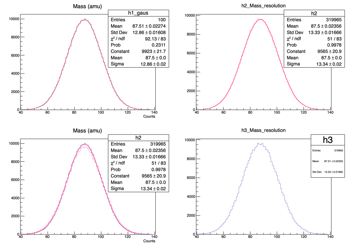
As you can see in the picture the sigma of h2 and h3 is more less equal to sqrt(3.5^2 +12.86^2 ) ~ 13.34, as expected.

I hope to have been clear in my explenation.

for(int j = 0; j < TMath::Nint(x); j++) {

Thanks, @Dilicus and @Wile_E_Coyote for the clear explanation. I understand now why my plots were showing Bizzard values for std after smearing.

I am a bit curious now as to whether it’s possible to do exactly the reverse of smearing ie., whether it is possible to eliminate the effect of smearing on the experimental data. Through simulation, I know my experimental mass resolution is say, 3.5 amu. By any means in Root is it possible to find my real or true mass distribution (by eliminating my effect of resolution on my experimental data, say for each of the mass data points in the experimental mass histogram)?

You can obtain the values of the initial distribution like the sigma, µ and amplitude, but you cannot get the initial data before the smearing.

Below you find a code to find the initial values.
The codes use the convolution of the initial distribution with the gaussian for the resolution, and I use the convolution function created with TF1Convolution to fit the smeared data.

There is another example here

void macro()
{

    
    auto h1 = new TH1D("h1_gaus","Mass (amu);Counts",101.0,39.5,140.5);
    auto h1_smeared = new TH1D("h1_gaus_smeared","Mass (amu);Counts",101.0,39.5,140.5);
    double amu=0;
    for(long int i=0;i<320000;i++)
    {
        //generate the original data µ=87.5, sigma 12.86
        amu=gRandom->Gaus(87.52,12.86);
        //fill the histo with the original distribution 
        h1->Fill( amu );
        //fill the histo with the smeared distribution 
        h1_smeared->Fill( amu + gRandom->Gaus(0,3.5));
    }
    
    //define a TF1Convolution, note that the range is slightly larger than the original one
   // the 2 functions are both gaussians, the first is your original distribution while the latter is
  // for the resolution
    TF1Convolution *f_conv = new TF1Convolution("gaus", "gaus", 30.,150., true);

    f_conv->SetRange(30.,150.);
    f_conv->SetNofPointsFFT(1000);
    //I create a TF1 from the TF1Convolution
    TF1 *f = new TF1("f", *f_conv, 40., 140., f_conv->GetNpar());
    //I create a gaussian for the unsmeared distribution 
    TF1 *f_gaus = new TF1("f_gaus_original","gaus", 40., 140.);
    
    // I set reasonable parameters for the convoluted function
    f->SetParameters(1e4,90.,13., 0.,3.5);
    // I fix the mean and the sigma of the gaussian accounting for the resolution 
    f->FixParameter(3,0.);
    f->FixParameter(4,3.5);
    
    TCanvas *c = new TCanvas("c","c",800,1000);
    c->Divide(1,2);
    //I draw the original histogram in the top part 
    c->cd(1);
    h1->Draw();
     //I draw the smeared histogram in the bottom part 
    c->cd(2);
    h1_smeared->Draw();
   // I fit the smeared histogram with the convolution function
    h1_smeared->Fit(f);
    
    
    c->cd(1);
    //I use the parameters of the convoluted function found with the fit to initialize the value of the original gaussina
    f_gaus->SetParameters(f->GetParameters());
    double convoluted_gauss_area= 3.5*TMath::Sqrt(2*TMath::Pi());
    //I need to rescale the amplitude parameter with the area of the convolution function
    //This is due the math property of convolution
    f_gaus->SetParameter(0,convoluted_gauss_area*f_gaus->GetParameter(0));
   // Here I just draw the gaussian on the original histogram, I not use any fit
    f_gaus->Draw("same");
       
}

Here you found the results of the fit obtained with the convolution function
As you can see p1 (µ) and p2(sigma) are very close to the one I used to fill the initial histogram (µ=87.52, sigma= 12.86). Note also as p3 and p4 are fixed.

FCN=123.174 FROM MIGRAD    STATUS=CONVERGED     123 CALLS         124 TOTAL
                     EDM=2.30469e-09    STRATEGY= 1      ERROR MATRIX ACCURATE 
  EXT PARAMETER                                   STEP         FIRST   
  NO.   NAME      VALUE            ERROR          SIZE      DERIVATIVE 
   1  p0           1.13228e+03   2.51851e+00   1.08943e-02   6.24005e-06
   2  p1           8.75508e+01   2.36011e-02   1.28403e-04  -2.38911e-03
   3  p2           1.28588e+01   1.73945e-02   7.52388e-05   2.55143e-03
   4  p3           0.00000e+00     fixed    
   5  p4           3.50000e+00     fixed 

Here the plot obtained.

When I run the macro I get the following error :

Take a pre-compiled binary distribution provided by the ROOT team (they should have the fftw3 feature enabled).

1 Like

Once again thanks @Dilicus.

I have a few doubts. Just to be sure that we both are on the same page, what I wanted to do was, I have experimental data (in which the effect of resolution is there), from the experimental data I want to have the true value say the mean and std of the distribution (without the resolution inside). So the following are my doubts :

  1. Does this method work if my experimental data deviates from a Gaussian function ? For better understanding here I attach my Experimental data which is gaussian like shaped but cant be fitted using a single gaussian function.
    Analysis.root (1.4 MB)

  2. Why is the mean value of the Gaussian accounting for the resolution is fixed to 0 ? As far as I understand for incorporating the resolution each points (mass bins) needs to be given a width of 3.5, so in this case the mean has to be the corresponing bin centers right ?

  3. Here I attach my macro using the experimental data using your method:

void Re_Smear()
{

gStyle->SetOptStat(2211);
gStyle->SetOptFit(1111);

/////////////////// Tree opening \\\\\\\\\\\\\\\

TFile *file1=TFile::Open(“Analysis.root”);
TTree tree1=(TTree)file1->Get(“Analysis”);

TH1D*h1 = new TH1D(“h1”,“h1”, 101.0,39.5,140.5);

//Defining a TF1Convolution
TF1Convolution *f_conv = new TF1Convolution("gaus", "gaus", 30.,150., true);

f_conv->SetRange(30.,150.);
f_conv->SetNofPointsFFT(1000);


TF1 *f = new TF1("f", *f_conv, 40., 140., f_conv->GetNpar());    
f->SetParameters(1e4,88.5,13.02, 0.,3.5); 
f->FixParameter(3,0.);
f->FixParameter(4,3.5);

TCanvas *c1 = new TCanvas(“c1”,“Without constraint”,800,600);
c1->Divide(2,2);
c1->cd(1);
tree1->Draw(“M_Tot>>h1”);
c1->cd(2);
h1->Draw(“E1”);
h1->Fit(f);

auto h2 = new TH1D(“h2”,“h2_Mass_resolution”,101.0,39.5,140.5);
h2 = (TH1D*)f->GetHistogram();
c1->cd(3);
gStyle->SetOptStat(2211);
gStyle->SetOptFit(1111);
h2->Draw(“E1”);
}

So if the method works, does it mean that my real data without resolution has the following mean and widths :

Capture1

Hi @gini,
I will have a look at this.

  1. Yes the method should work. But this means also that the original distribution before being smeared by the resolution had two gaussian components.

  2. The value is 0 because the convolution process takes care to move the gaussian accounting for the resolution .

Yes the mean and width of the original resolution will be shown in the fit.

This is your modified code. I added limit parameters to the variables which are not fixed, and I put also option “ME”.
It should help the fit to converge, since is quite hard. It seems you have 2 gaussian very close to each other with a very similar \sigma, I also highlighted the 2 gaussians.
Re_Smear.c (2.0 KB)

I attach also a test code similar to the previous one where I use two gaussians with quite different \mu and \sigma. You can test it changing the parameters of the gaussian used to fill
macro.c (1.9 KB)

Hi @Dilicus ,

Yes you are right. The original distribution is reproduced using three Gaussian fitting, one at the mean value (black) and two others positioned equidistand from the center (green).

The histogram is fitted using the following function :

[0]exp(-0.5((x-[1])/[2])**2) + [3]exp(-0.5((x-([1]-[4]))/[5])**2) + [3]exp(-0.5((x-([1]+[4]))/[5])**2)

Thanks for the consideration !

I changed my code to use 3 gaussians like you did , I just payed attention to keep the variable related to the convolution function fixed.

The result should be quite similar since the number of free parameters is the same.
Re_Smear_3gauss.c (1.7 KB)

Thanks @Dilicus for the modified macro.

So if I understand you correctly the real width of my distribution (with no resolution) is 12.98 amu, which is the width of the convolution function which we used to fit the experimental data, with resolution inside.

Yes you are correct.
To be sure we are understanding each other, the real width is the width of the first function inside the TF1Convolution (the sum of the 3 gaussian).
PS
For me the original width is slightly different. It is 12.896

So to be clear about the widths:

The width of my distribution with resolution inside ie.,
Experimental Mass Width = 13.02 (which is also represented using the first function inside the TF1Convolution ie., the sum of 3 gaus)

The width of the distribution without resolution = Width of the function used for fitting = 12.98
I don’t know why the values are different. But I really wonder if this is true as the function used for fitting is derived from the convolution function and in the convolution function the effect of the resolution is there.

Previously when we considered the convolution function to be two gausses ie., one for the distribution and the other to account for the resolution, the widths that we obtain from the fitting data keeping the fit parameters of resolution fixed were fine. But since now we use the sum of gaussian functions to represent the experimental data i don’t think the width without resolution is equal to the width of the convolution function. please correct me if I am wrong.

I think I finally got precisely what you want.
It will took times, but I will try to explain all the details.

You fit your data with a function f which is the convolution of two other functions, so is defined as

f_{conv}=(f) * g(x) =\int_{-\infty}^{+\infty} f(x-\tau) g(\tau) d\tau

in your case the first function f is the sum of 3 gaussians and g is the gaussian for the resolution

So

  • f this is the shape of your data before being affected by the detector resolution, this is the sum of 3 gaussians, you are searching the width of f.
  • g this the resolution function, is a gaussian
  • f_{conv} this is the shape of the data you collected after the effect of the detector resolution , you have this width

Your experimental mass width is the std dev computed by root when filling the histogram and is computed indicated in TH1::GetStdDev(), and since there are no overflow and underflow the Std Dev in the Histogram stats is correct.

Then in your code after fitting the distribution with you want to generate an histogram and looking at the standard deviation of such histogram in the stats you want estimate the width of the original distribution

This is correct but if you generate the histogram using f_{conv} you will have the same width.
If take in account the errors 13.02 and 12.98 are basically the same number.

Instead after the fit you should generate the histogram using only f. From the fit you need to extract the info of f and use f to generate the histogram
I modified the code
Re_Smear_3gauss.c (1.9 KB) so that work in the right direction and the width of resulting the distribution in ~12.5.

To compare with the result expected from a simple computation

\sigma_{0}=\sqrt{\sigma^2_{data} - \sigma^2_{res}} = \sqrt{13.02^2 -3.5^2}\simeq12.5

PS
In the code I normalized the integral of g so that the amplitude of f from the fit is not changed by the effect of the convolution

Now it all makes sense @Dilicus . What I don’t understand is how you fix the amplitude of the smeared Gaussian and is it necessary to do so ?

Also when I plot in c1->cd(1) I just want to plot the histogram “h1” without the fitting it, is it possible to do so ?