Hello everyone, I’m new to ROOT. I need some help learning Monte Carlo methods, and I’m very much stuck. I need to use the Central limit theorem and Box-Muller methods to generate random numbers distributed as a Gaussian pluck from a string wave problem and then use the ROOT fitting to test my results. Can someone please give me some advice on how to start or recommend some readings on the topic? Thank you so much for your help. I really appreciate it.
Hi @lila,
welcome to the ROOT forum!
So you should generate random Gaussian numbers first using the central limit theorem, and then using the Box-Muller method, is that right?
I can give you an example on how you can generate a single random Gaussian number from n independent uniform ones, exploiting the Central Limit Theorem (CLT). Maybe it serves as an inspiration, and you can adapt this to try the Box-Muller method.
// Generating random Gaussian numbers by adding random uniform
// numbers and relying on the central limit theorem for this to converge
// to a Gaussian when we add many independent uniform numbers.
// Fit the resulting histogram with a Gaussian as a crosscheck.

void central_limit_method() {

    // Create histogram with 200 bins from -4 to 4
    auto hist = new TH1D{"hist",
                         "Random Gaussian numbers (CLT)",
                         100, -4, 4};

    // How many random numbers we generate
    std::size_t nEntries = 10000000;

    // Number of random uniform variables we sum up to get a Gaussian
    // in the limit according to the central limit thoerem
    int nVariables = 30;

    // Instantiate ROOT's TRandom3 random number generator
    TRandom3 rng;

    for(std::size_t i = 0; i < nEntries; ++i) {

        double val = 0.0;
        for(int iVar = 0; iVar < nVariables; ++iVar) {
            val += rng.Uniform();
        }
        // normalize, considering the mean and the variance of the
        // uniform variables, see:
        // https://en.wikipedia.org/wiki/Continuous_uniform_distribution
        val -= 0.5 * nVariables;
        val /= std::sqrt(nVariables * (1./12.));

        // Fill the histogram
        hist->Fill(val);
    }

    // Fit the histogram with a Gaussian to verify the sum of
    // uniform random variables is indeed Gaussian in the limit:
    hist->Fit("gaus");

    // To get the fit parameters in the plot
    gStyle->SetOptFit();

    // Draw the histogram with the fit
    hist->Draw();

}
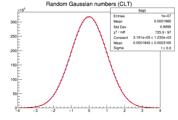
Just put this in a file called central_limit_method.C and run it by typing root central_limit_method.C in the terminal. You should get this plot.
Hope this helps to get started! If you need further inspiration, I can also advise you to take a look at the ROOT tutorials. Also, don’t hesitate to ask further questions in this thread.
Cheers,
Jonas
Hi @jonas ,
Thank you so much for your answer. It really helped me a lot to get started.
What I don’t understand yet, is how we can normalize a function considering the mean and the variance without explicitly writing out the code:
val -= 0.5 * nVariables;
val /= std::sqrt(nVariables * (1./12.));
but instead using some code/function that would normalize a histogram? I’m asking this because I’m struggling to normalize multiple histograms and I guess that code would help a lot.
Thank you again for all your help.
Best,
Lila
Hi @lila!
some code/function that would normalize a histogram
Can you be more specific of what you want to achieve? With “histogram”, do you mean a ROOT TH1 object? Then, remember that the values are already binned. How would you expect the binning to change when normalizing the histogram? You would expect a new histogram with a new binning scaled by your normalization factors, or a histogram with the same binning where the values are re-filled to be normalized? In the latter case, you would definitely suffer from binning effects.
So it’s better to normalize the values before filling the histogram, instead of normalizing the histograms where you get in trouble with the binning.
Here is how I would do it, based on the example in my initial answer:
void normalize(std::vector<double> & values) {
    double mean = 0.0;
    double vari = 0.0;

    // first pass: get the mean
    for(std::size_t i = 0; i < values.size(); ++i) {
        mean += values[i];
    }
    mean /= values.size();

    // second pass: get the variance
    for(std::size_t i = 0; i < values.size(); ++i) {
        double tmp = values[i] - mean;
        vari += tmp * tmp;
    }
    vari /= values.size();
    // compute the inverse standard deviation so we can do multiplicatin in the
    // loop, which is faster than division
    double sinv = 1./std::sqrt(vari);

    std::cout << mean << std::endl;
    std::cout << vari << std::endl;

    // final pass: normalize the values
    for(std::size_t i = 0; i < values.size(); ++i) {
        values[i] -= mean;
        values[i] *= sinv;
    }
}

// Generating random Gaussian numbers by adding random uniform
// numbers and relying on the central limit theorem for this to converge
// to a Gaussian when we add many independent uniform numbers.
// Fit the resulting histogram with a Gaussian as a crosscheck.

void central_limit_method_2() {

    // Create histogram with 200 bins from -4 to 4
    auto hist = new TH1D{"hist",
                         "Random Gaussian numbers (CLT)",
                         100, -4, 4};

    // How many random numbers we generate
    std::size_t nEntries = 10000000;

    // Number of random uniform variables we sum up to get a Gaussian
    // in the limit according to the central limit thoerem
    int nVariables = 30;

    // Instantiate ROOT's TRandom3 random number generator
    TRandom3 rng;

    std::vector<double> values(nEntries);

    for(std::size_t i = 0; i < nEntries; ++i) {

        double val = 0.0;
        for(int iVar = 0; iVar < nVariables; ++iVar) {
            val += rng.Uniform();
        }

        values[i] = val;
    }

    // Normalize the values
    normalize(values);

    for(std::size_t i = 0; i < nEntries; ++i) {
        hist->Fill(values[i]);
    }

    // Fit the histogram with a Gaussian to verify the sum of
    // uniform random variables is indeed Gaussian in the limit:
    hist->Fit("gaus");

    // To get the fit parameters in the plot
    gStyle->SetOptFit();

    // Draw the histogram with the fit
    hist->Draw();

}
By the way, these kind of array operations can be done very conveniently in Python with NumPy. Have you considered using Python for your work? You can also use ROOT from Python too.
Cheers,
Jonas