How to fit a skew gaussian?

Hello everyone,

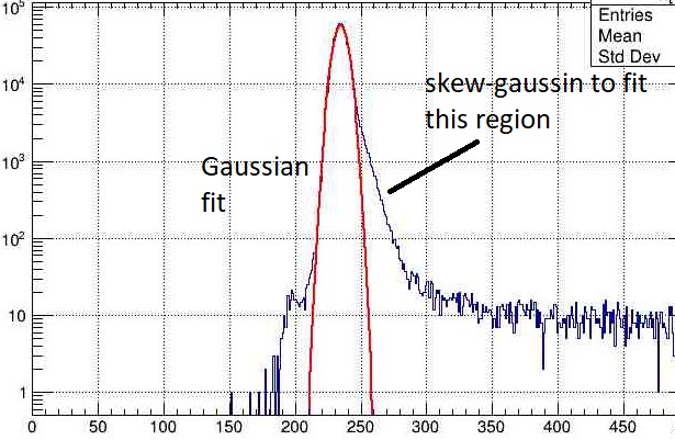
How can I fit the skew-gaussian on the histogram plot. As one can notice in the attached plot, I tried to fit the gaussian curve but lots of counts are not covered by the gaussian.

I referred to the wikipedia page of skew-gaussia (Skew normal distribution - Wikipedia) but as the formula involves the integration, I don’t know how to implement it in ROOT.

Any suggestion would be a great help.

Thanks,
Divyang.

can6

Hi @Divyang!

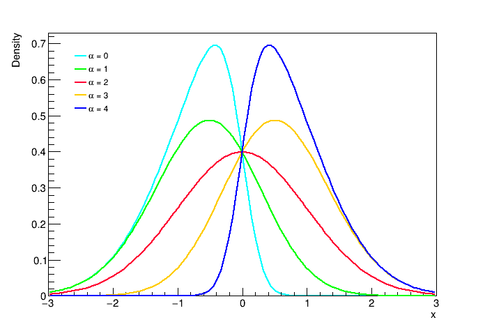
No big deal with the integral, as you can also read on Wikipedia in the “Definition” section. You can formulate the PDF in terms of the error function, which is also available in ROOT or standard C++ (std::erf). With this script I can reproduce the figure from Wikipedia, for example:

// testSkewedgauss.C

double skewedgauss(double * x, double *p) {
    double xi = p[0];
    double omega = p[1];
    double alpha = p[2];
    double arg = (x[0] - xi) / omega;
    double smallphi = TMath::Gaus(arg, 0.0, 1.0, true);
    double bigphi = 0.5 * (1 + std::erf(alpha * arg/std::sqrt(2)));
    return 2./omega * smallphi * bigphi;
}


void testSkewedgauss() {

   std::vector<double> shapes{-4.0, -1.0, 0.0, 1.0, 4.0};
   std::vector<int> colors{kCyan, kGreen, kPink, kOrange, kBlue};

   auto c1 = new TCanvas();
   auto legend = new TLegend(0.15,0.65,0.28,0.85);
   legend->SetBorderSize(0);

   for(std::size_t i = 0; i < shapes.size(); ++i) {
      std::string name = "f" + std::to_string(i);
      TF1 *f = new TF1(name.c_str(), skewedgauss,-3.0, 3.0, 3);
      f->SetTitle(";x;Density");
      f->SetParNames("location","scale","shape");
      f->SetLineColor(colors[i]);
      f->SetParameters(0.0, 1.0, shapes[i]);

      f->Draw(i == 0 ? "" : "SAME");
      auto label = "#alpha = " + std::to_string(i);
      legend->AddEntry(name.c_str(),label.c_str(),"l");
   }

   legend->Draw();
   c1->Draw();

   c1->SaveAs("skewedgauss.png");
}

Hope this helps!
Jonas

1 Like

Thanks, @jonas!

I didn’t know about the erf function. ROOT is very powerful :muscle: :fist:.

Thanks again,
Divyang.

Just want to mentioned that these curves are normalized. Hence, I added one more parameter, amplitude. Here is the function I used for fitting the histogram I mentioned in the question,

double Skewed_Gauss(double *x, double *p)
{
  double shift     = p[0];   // first argument is shift
  double spread    = p[1];   // second argument is spread
  double skewness  = p[2];   // third argument is skewness
  double amplitude = p[3];   // fourth argument is amplitude

  double argument = (x[0] - shift)/ spread;

  double Norm_gaus = TMath::Gaus(argument, 0.0, 1.0, true);
  double CDF       = 0.5 * (1 + erf(skewness* argument/sqrt(2)) );

  return amplitude* Norm_gaus* CDF;
}

See also:

and:

https://root.cern/doc/master/langaus_8C.html