Fitting with a multiplication series and factorial

[Rahul]

Hello Experts,

I am trying to fit a distribution with the following form of equation:

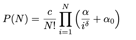
I made the following code for the purpose:

double myFitFunction(double *x, double *p)//Subpossonion
{

    int N = (int)std::round(x[0]); 
    double mul =1.0;
    for (int i = 1; i < N; ++i)
    {
      mul = mul*((p[2]/pow(i,p[3]))+p[1]);
    }
    
    double r = p[0]*mul/tgamma(x[0]+1);

    return r;
}


void CrossCheck()
{
  
  
    gStyle->SetOptStat(1);
    gStyle->SetOptFit(1);
    gStyle->SetTitleW(0.4);
  
    
  //Histogram
   TCanvas* canvas = new TCanvas();
   canvas->SetLogy();
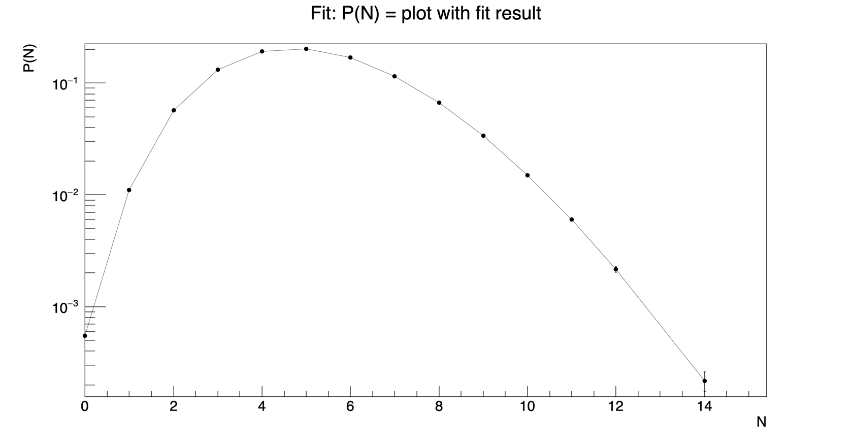
   double binY[14]  = {0.00055, 0.01083, 0.05802, 0.1293, 0.1917, 0.2019, 0.1692, 0.1151, 0.06641, 0.03329, 0.014690, 0.006080, 0.002279,0.0003763};
   double binYE[14] = {0.00000, 0.00019, 0.00042, 0.0006, 0.0007, 0.0008, 0.0008, 0.0007, 0.00055, 0.00043, 0.000300, 0.000188, 0.000132, 4.31e-05};
   double binX[14] = {0.,1.,2.,3.,4.,5.,6.,7.,8.,9.,10.,11.0,12.0,14.0}; 
   double binXE[14] = {0.};

    TGraphErrors* Summation = new TGraphErrors(14,binX,binY,binXE, binYE);
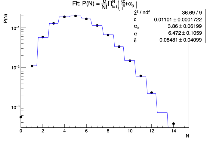
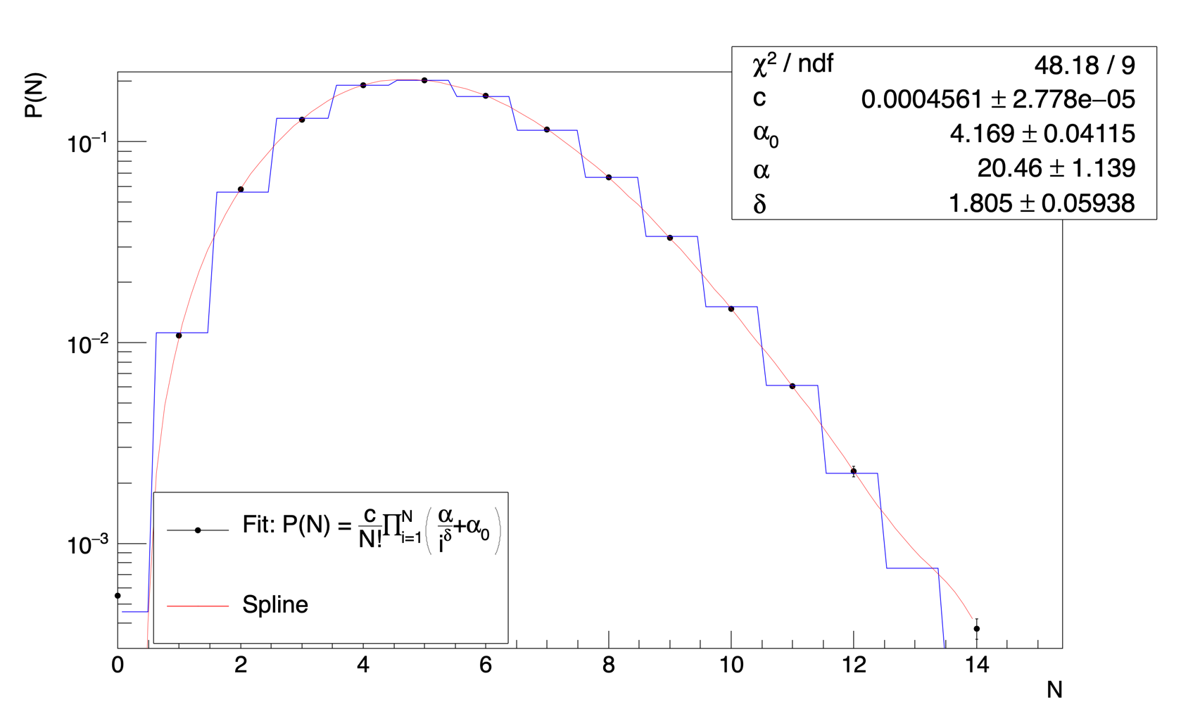
    Summation->SetTitle("Fit: P(N) = #frac{c}{N!}#prod_{i=1}^{N}(#frac{#alpha}{i^{#delta}}+#alpha_{0})");
    Summation->GetYaxis()->SetTitle("P(N)");
    Summation->GetXaxis()->SetTitle("N");
    Summation->SetMarkerColor(1);
    Summation->SetMarkerSize(1);
    Summation->SetMarkerStyle(20);
    Summation->Draw("AP"); 
 
   TF1 *fitMul =new TF1("fitMul",myFitFunction,0,14,4);
   fitMul->SetParLimits(0,0.0,1.00);
   fitMul->SetParLimits(1,1.0,10.0); 
   fitMul->SetParLimits(2,0.0,150.);
   fitMul->SetParLimits(3,0.0,10.0);
   fitMul->SetParNames("c","#alpha_{0}","#alpha", "#delta");
   fitMul->SetLineColor(4);
   fitMul->SetLineWidth(2);
   //Do Fit
   Summation->Fit(fitMul,"RME"); 

}

which gives the following fit curve:

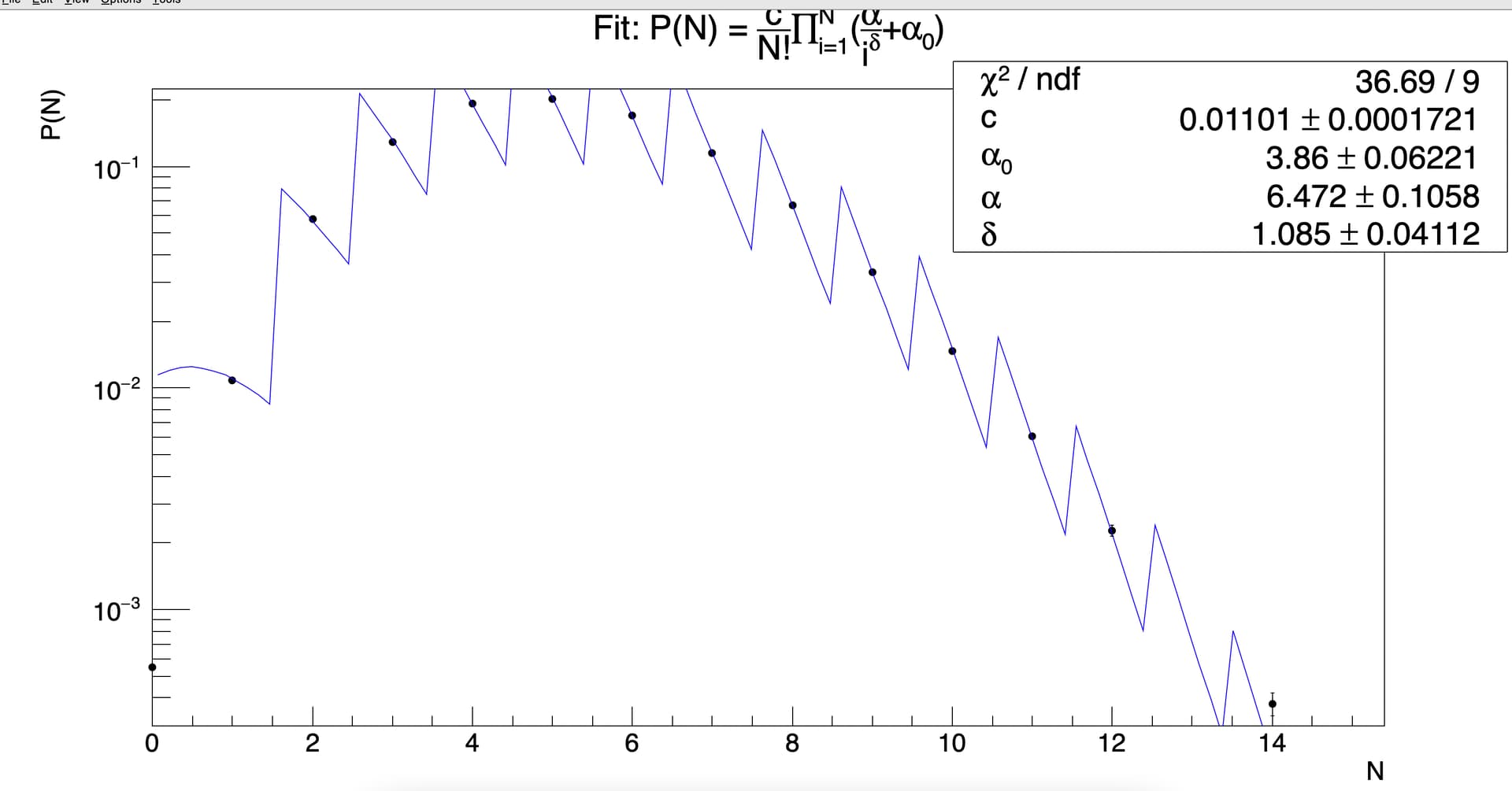
Since the multiplication series is from i = 1 to N and there is N! which has to be taken from the X axis during the fitting, I did this:

int N = (int)std::round(x[0]);

and I am using:

n! = tgamma(n+1)

in the fit function. I think that something is obviously wrong with the way in which I am trying to implement this fitting. Could you please help me to make it correct?

Sincerely
Rahul

[Wile_E_Coyote]

double r = p[0]*mul/tgamma(N + 1.);

[Rahul]

Hi,

Thank you for the suggestion. I tried that and I get the following plot:

It is supposed to give a smooth curve as per the publications. So I am still confused.

When a slightly simpler form of P(N) was used (with a separate user-defined function as in the code) which did not include the multiplicative series, I got a similar step-like curve earlier. While the same simple form of P(N) gave a smooth curve when I try to fit it in a similar fashion like this:

TF1 *fitMul = new TF1("fitMul","0.229*TMath::Power([0],x)/TMath::Power(TMath::Gamma(x+1),1+[1])",1,27);

Hence I was wondering whether there is still some mistake in the form of implementation in my code.

Sincerely
Rahul

[Wile_E_Coyote]

Your “P(N)” is, by definition, a “step-like” function.
You need to define a function that is “smooth”.

[Rahul]

Hi,

If I plot the graph with the fit result from the previous fit using the “APL” option, it gives the following figure:

The form of P(N) I mentioned was used for fitting in PRD 105 (2022) 054003 (arXiv PDF) [ Figure 5, Equation 21] which in fact shows a smooth curve.

Sincerely
Rahul

[Wile_E_Coyote]

You need to ask the authors of this paper why they cheat.
The “Equation 21” is defined for positive integer values “N >= 1” (the “smooth” curve could be some interpolated “spline”).

[smgrig]

@Rahul

for (int i = 1; i < N+1; ++i)

use N+1 in your “for loop”

[Wile_E_Coyote]

Yeah, I missed it (that’s why the first bin was missing): for (int i = 1; i <= N; ++i)

[Rahul]

Hi @smgrig @Wile_E_Coyote ,

Thanks a lot for your comments and suggestions. I changed the for loop to this:

for (int i = 1; i <= N; ++i)

and I tried to draw a spline with this:

   TSpline3 *s = new TSpline3("Spline",Summation);
   s->SetLineColor(kRed);
   s->Draw("same");

The result is shown below:

P(0) is not actually a data point but is obtained from the extrapolation of a model to N =0. But I think the issues with my fitting are solved now.

Thank you
Rahul

[Wile_E_Coyote]

If you plan to work on it, I think you should ask the authors of this pager what they do, how, and why.

[Rahul]

@Wile_E_Coyote : They were making the modified combinants Cj from the experimental P(N) distribution and performing fit on the Cj with phenomenological models of particle production with the argument that the same distribution that fits P(N) is not suitable for the obtained Cjs. Hence in order to get additional information about the production processes, a Cj-based analysis has to be made. Additionally, some of the other aspects of Cjs were also studied by them. So the fitting in their case started with Cjs, not P(N). But I agree that the caption in the particular paper I mentioned was misleading. I always was keeping Chi^2/NDF ~ 1.0 as a measure in my mind to proceed further or not with the fit results. But this one got me into trouble.

[Wile_E_Coyote]

I did not read this paper, but most plots have “N” on the x-axis, which I assume are “integer values” by definition. However, they always draw “smooth curves”, so you should ask them how they get them (and what is the meaning of noninteger “N” values).

Playing with “splines” may be dangerous.
For example, if you calculate integrals somewhere, for the “step-like” function, the integral inside of a bin is just its value at the bin center (because the bin width is 1). However, if you integrate the “spline” inside of a bin, you may get a very different value (sometimes bigger, sometimes smaller than the “correct” value from the bin center).

[Rahul]

@Wile_E_Coyote: Sure, I shall do that and I also agree with your points about using splines. Thank you for the comments indeed. I shall keep it in mind. The N is the number of particles and hence are positive integers. But I was having this idea in mind that we get smooth curves for P(N) (albeit I understand the form of P(N) here is different). But generally, smooth curves are obtained for P(N) plots while fitting with 1-NBD, 2- NBD etc. Eg: Figures 3, 4, and 5 in the ALICE paper: Eur. Phys. J. C (2017) 77:852 (PDF) and many more papers. Hence I did not even think about the step-like function at all when I started to fit it.

[Wile_E_Coyote]

Again, I did not read this second paper, but the equation “(6)” for “P_NBD(n, <n>, k)” is well defined also for noninteger parameters, and it even explicitly has a noninteger (by definition) parameter “<n>”, so I think it can be “smooth”.
So, this is very different from the first paper.

BTW. If you look at “Fig.6” and “Fig.7”, you can clearly see that the curves are drawn “step-like”.

[Rahul]

Yes, I also thought that because of the real-valued parameters alpha and alpha 0 in the P(N) I have used, the P(N) could be smooth without thinking about it further (The SetParLimits() had real-valued intervals). The curves Fig. 6 and Fig 7 in Eur. Phys. J. C (2017) 77:852 are not actually coming from the fit but they are experimental (or simulated with MC generators) data points I think. They just connected the bin edges I guess and have very small error bars due to large statistics for the MC data.

[Wile_E_Coyote]

@Rahul

They just connected the bin edges

I just wanted to say that they used the "E" and "HIST" (“step-like”) drawing options, and they did not use the "L" nor "C" drawing options (which would create a “semi-smooth” curves through the histogram bins).
So, using “step-like” functions makes sense, too.

[Rahul]

I see. I understood, thanks. What I am bothered about now is the Chi^2/NDF value that I would be getting in such a case.

[Wile_E_Coyote]

Well, the “chi^2” is anyhow calculated at data points, so it doesn’t depend if the function is “step-like” or “smooth” (it simply calculates its value at these points), and the “ndf” is just the number of data points minus the number of function parameters.

[Rahul]

OK. Unless some great mistakes are hidden in my code, I think it altogether solves my problem with this type of fitting. Thanks a lot!

[Wile_E_Coyote]

As you use “round”, you could probably define your function with xmax = 14.5 (instead of 14), so that the last “full step” is 13.5 to 14.5 (this shouldn’t change fit results).