I am currently performing an unbinned maximum likelihood fit to extract two parameters (a1, a2) from N events. The likelihood function is constructed as:
-lnL=Sum_{i=0}^{N} ln W(\xi_i; a1,a2)
I then attempted to incorporate a constraint between a1 and a2 using the Lagrange multiplier method, modifying the likelihood function to:
However, when minimizing -lnL using TMinuit, the fit consistently hits the boundary regardless of how I adjust the range of lambda, resulting in failed convergence. I would like to ask:
Whether my construction of the likelihood function using the Lagrange multiplier method is correct
Whether TMinuit is an appropriate tool for this constrained minimization approach
Sorry for the late reply as I was away attending a conference.
I will promptly try the Gaussian constraint approach as you suggested.
Regarding error propagation for fixed parameters, I also implemented it by performing multiple fits while varying the values of the fixed parameters.
Would it be possible for you to share the relevant code if convenient?
where likelihood_F(x) is the negative log likelihood estimator, and std::log( ... ) is the constraint.
I am not a great expert, but I suspect that the result might be biased when adding constraints, so please try at least with some synthetic data (where you know the parameters) similar to your experimental data, to crosscheck that your method is still robust and non-biased (check the pulls)
I would also go for a Gaussian constraint, thanks @atd!
And just to not discourage you from using the constraint, I would not call the fit “biased”, because if you know (due to external physics knowledge or similar) that there needs to be a relation between the parameters, you are actually giving the minimiser more information, which it couldn’t know otherwise.
I wanted to ask a follow-up from a more mathematical/statistical perspective:
Suppose I generate many synthetic datasets using a known model and known true parameter values, and then fit each dataset by minimizing a likelihood function plus Gaussian constraints. Is it mathematically guaranteed that this estimator will have these properties?
Unbiased, i.e. the average of the fitted parameters over many pseudo-experiments converges to the true values?
Consistent, i.e. the variance of the estimator decreases as the number of events increases?
Or, from other perspective: under what conditions can we say that adding such Gaussian constraints (assuming they’re centered on the correct values) still yields asymptotically unbiased and consistent estimates?
Thanks in advance for your thoughts, I’m trying to get a deeper understanding of when these techniques are robust.
we would better refer this question to somebody with deeper knowledge in statistics like @moneta.
That being said, if you add a Gaussian constraint on a parameter, it depends to what value you constrain it. You will clearly bias a fit if you generate a dataset with some parameter a=-10, but then you constrain it to a=0±1. Clearly, an unbiased fit model without the constraint should converge to -10, whereas a fit with constraint will be pulled towards 0.
But in most cases, that’s not what we are doing. We usually generate toy data with some value of a, but then we constrain a to the same value when fitting. And moreover, we add constraints mostly on parameters that the fit model isn’t very sensitive to. We want to avoid them to assume values that seem somehow random, and therefore we add information from external measurements using those constraint terms. If our fit is already very sensitive to the parameter, there is no real need to constrain it.
In HEP we therefore have the “parameter of interest” and the “nuisance parameters”: We measure the parameter of interest, and we constrain nuisance parameters (the ones we don’t want to measure directly) to values that we found in external measurements.
To come back to your questions:
If you add a constraint at the correct central value and with the correct variance, you are actually helping the fit model to be unbiased and consistent. When you generate toy datasets, you should actually generate them with the constraint terms active, so you get a “realistic” distribution.
This will of course break down if one of your constrained parameters is not Gaussian in nature. In that case, you can add other constraints, such as Poisson or LogNormal, or (the most accurate way but not always feasible) you simply multiply the likelihood function of your main measurement with the likelihood function of your external or auxiliary measurement, which will allow you to perform a combined measurement of the two, or of many parameters simultaneously.
Since this is either cumbersome or slow, or both, we often “approximate” the auxiliary likelihood functions with a Gaussian around whatever value the auxiliary measurements produced. So in that sense, the preferred order in terms of accuracy and predictive power is:
The “super likelihood” with all measurements, main and the auxiliary ones, multiplying all likelihood functions of all measurements.
The second best is to create the main likelihood model and add constraint terms for the auxiliary measurements, getting very close to the real thing if the errors of your auxiliary measurements are Gaussian.
And the worst is to have the main likelihood without any constraint terms, completely missing the external information.
Sorry for the late reply. I tried using Gaussian-shaped constraints in the likelihood equation, but ultimately failed. Similarly, during minimization, lambda reached the boundary. My fitting procedure is as follows: AngularFit.C (7.7 KB)
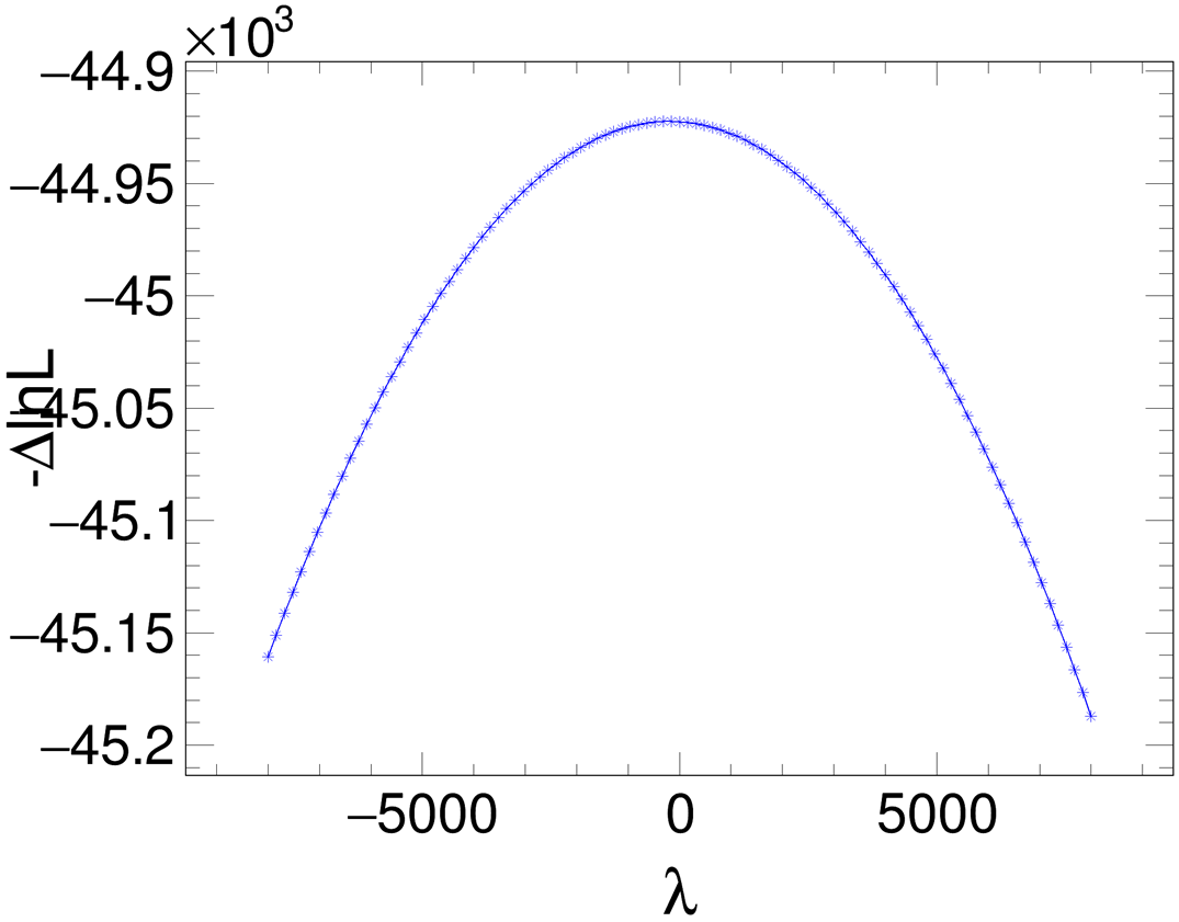
I’m not an expert in fitting, but I have a conjecture about this issue: Since the lambda multiplier is linear in the likelihood function, if the constraint is not strictly zero during fitting, then minimizing the likelihood will exhibit monotonic behavior with respect to lambda. As a result, the likelihood can only reach its minimum when lambda hits the boundary.
I’m not entirely sure whether this understanding is correct, so I also performed a scan of the likelihood function over the lambda multiplier. Indeed, the results show that the likelihood only reaches its minimum when lambda is at the boundary—its extremum at lambda=0 is not the minimum point.
I attempted an alternative approach using the Augmented Lagrangian Method. The likelihood function is constructed as follows:
S=S_{Nom} + lambda * g(Omega) + rho * g(Omega)^2
where S_{Nom} is the likelihood function without constraint, g is constraint function, Omega is the fitted parameters, lambda is the Lagrange multiplier and rho is the penalty coefficient. In this fitting procedure, lambda (λ) and rho (ρ) are not treated as free parameters in the TMinuit minimization, but rather as external control parameters . We need to perform a series of iterations, where in each iteration:
Fix lambda_{k} and rho_{k}, solve the unconstrained problem by TMinuit:
Parameter Omega_{k} = min S_{Nom}
Update the penalty coefficient rho_{k}:
rho_{k+1} = 2 * rho_{k}
Termination criterion for iterations: |g(Omega)| < epsilon, where epsilon is the predefined tolerance, set to 1e-6.
Through this approach, the expected results were successfully obtained after 16 iterations. I would like to inquire whether this method can be widely applied to constrained optimization problems in general.
Best,
Yupeng
Reference:
[1] Hestenes, M.R. (1969) Multiplier and Gradient Methods. Journal of Optimization
Theory and Applications, 4, 303-320.
[2] Powell, M.J.D. (1969) A Method for Nonlinear Constraints in Minimization Prob
lems. In: Fletcher, R., Ed., Optimization, Academic Press, New York, NY, 283-298.
[3] Bertsekas, D.P. (1996) Constrained Optimization and Lagrange Multiplier Methods.
Athena Scientific (First Published 1982).