Cubic polynomial fit 4 points has uncertainties


Please read tips for efficient and successful posting and posting code

ROOT Version: 6.18.04
Platform: Linux
Compiler: gcc


Hi,

Could anyone help me to explain why I got uncertainties when I fit 4-point graph with cubic polynomial? The following is my brief code:

void MyTest()
{
    double x[4] = {528, 529, 530, 531};
    double y[4] = {813.128, 690.941, 592.383, 413.539};
    TGraph *gr = new TGraph(4, x, y);
    gr->Draw("AP*");
    gr->Fit("pol3");
}

Because there are four points, in principle the four parameters of cubic function should be determined without any uncertainties. But I do get the uncertainties. Why?

Thank you!

Hi,

The uncertainties are computed from the parameter values giving a Delta(chi2) = 1, so also in case of 0 degree of freedom, they will not be zero.
However, I see that the function does not pass through the points, you see the chi2 is different than zero, this also shows that the solution is not valid, probably caused by a numerical error inverting the matrix. You should translate the x and y values to be closer to 1 and it will work.
For example for these x points it will work:

double x[4] = {28, 29, 30, 31};

Lorenzo

Hi Lorenzo,

Thank you. I tried to change x points as:
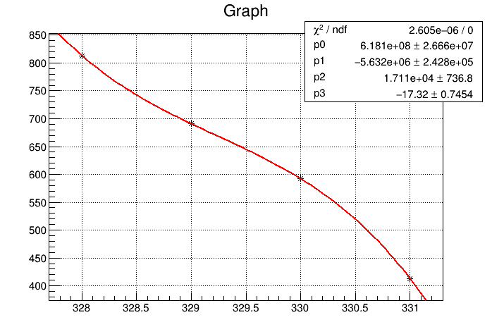
void MyTest()
{
    double x[4] = {328, 329, 330, 331};
    double y[4] = {813.128, 690.941, 592.383, 413.539};
    TGraph *gr = new TGraph(4, x, y);
    gr->Draw("AP*");
    gr->Fit("pol3");
}

And it looks wee now.


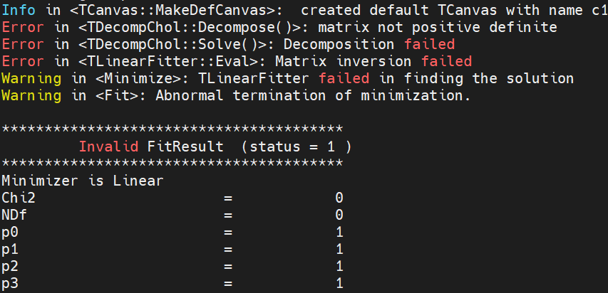
Then if I change x points by 100 more like:

void MyTest()
{
    double x[4] = {428, 429, 430, 431};
    double y[4] = {813.128, 690.941, 592.383, 413.539};
    TGraph *gr = new TGraph(4, x, y);
    gr->Draw("AP*");
    gr->Fit("pol3");
}

Then it gives me errors:

It’s strange. If I use MS-Excel or LibreOffice, I can easily get a correct results:

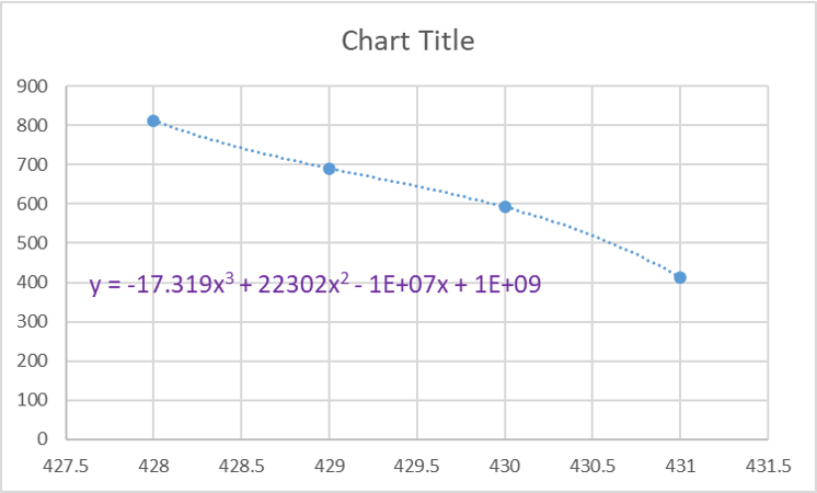
So how should I set ROOT to fit “pol3” to 4 points always correctly?

Thank you,
Kailong

Hi,

The trick is to keep the points close to 1 as much as possible. If you want a generic procedure, apply for example a translation and a scale to the x values such the first point is around 1 and the last one is at around 10.

Lorenzo

I tried:

{
  double x[4] = {8, 9, 10, 11};
  //double x[4] = {18, 19, 20, 21};
  //double x[4] = {28, 29, 30, 31}; // "Minuit / Migrad" FAILS
  //double x[4] = {38, 39, 40, 41}; // "Minuit / Migrad" FAILS
  double y[4] = {813.128, 690.941, 592.383, 413.539};
  TGraph *gr = new TGraph(4, x, y);
  ((TF1*)gROOT->GetFunction("pol3"))->SetParameters(0., 0., 0., 0.);
  gr->Fit("pol3"); // Minimizer is Linear / Migrad
  ((TF1*)gROOT->GetFunction("pol3"))->SetParameters(0., 0., 0., 0.);
  gr->Fit("pol3", "F"); // Minimizer is Minuit / Migrad
}

and the result is (note: the fitted parameters are equal but please compare their errors; can this be fixed somehow?):

****************************************
Minimizer is Linear / Migrad
Chi2                      =  1.41398e-17
NDf                       =            0
p0                        =      15111.1   +/-   626.132     
p1                        =     -4514.27   +/-   200.503     
p2                        =      479.432   +/-   21.2485     
p3                        =     -17.3192   +/-   0.745356    

****************************************
Minimizer is Minuit / Migrad
Chi2                      =  3.46746e-10
NDf                       =            0
Edm                       =  2.31219e-11
NCalls                    =          162
p0                        =      15111.1   +/-   4.41748     
p1                        =     -4514.27   +/-   0.695362    
p2                        =      479.432   +/-   0.070269    
p3                        =     -17.3192   +/-   0.0049434   

As soon as one tries “double x[4] = {28, 29, 30, 31};”, the “Minuit / Migrad” fails:

****************************************
Minimizer is Linear / Migrad
Chi2                      =  6.41198e-15
NDf                       =            0
p0                        =       435723   +/-   19094.9     
p1                        =     -44474.6   +/-   1944.63     
p2                        =      1518.58   +/-   65.9659     
p3                        =     -17.3192   +/-   0.745356    

****************************************
Minimizer is Minuit / Migrad
Chi2                      =      526.888
NDf                       =            0
Edm                       =    8.964e-06
NCalls                    =          152
p0                        =     -2554.59   +/-   5.37655     
p1                        =      162.318   +/-   0.227158    
p2                        =      4.40956   +/-   0.00766599  
p3                        =    -0.211349   +/-   0.000207833 

@Axel It seems to me that this simple example shows serious deficiencies of ROOT’s minimizers.

Thank you so much. It’s interesting and great to know that the polynomial fit is sensitive to the x value’s range and requires the scaling.

Probably, it would be better if the polynomial fit performs well without scaling x values then the fitting parameters could be used directly without any translation.

Kailong

Hi,
It is not the polynomial fit that is sensitive, it is whatever function you are using if your data are not well balanced. It is a limitation of using floating point computations and not infinite precision.

@Wile_E_Coyote : the example above Minuit fails and it is expected because you start with initial parameters (0,0,0,0) which are too far off from the minimum. Minuit is a local minimizer and if you start from a bad region there is no way it will converge.
In the case of the linear fitter (more sensitive to numerical precision when inverting the matrix) you don’t need to set any initial parameter values

@moneta Note that in the case when both minimizes converged (to the same minimum), they returned completely different errors (by two orders of magnitude at least). This should not be allowed (which errors are meaningful?).

The “initial parameters (0,0,0,0) which are too far off from the minimum” is a tempting hypothesis, of course.
However, for the “double x[4] = {28, 29, 30, 31};” case, I tried:

  ((TF1*)gROOT->GetFunction("pol3"))->SetParameters(4e5, -4e4, 2e3, -20);
  gr->Fit("pol3", "F"); // Minimizer is Minuit / Migrad

and it still failed:

****************************************
Minimizer is Minuit / Migrad
Chi2                      =      5.55195
NDf                       =            0
Edm                       =  1.00445e-07
NCalls                    =          146
p0                        =       480712   +/-   5.3762      
p1                        =     -49056.6   +/-   0.227149    
p2                        =      1674.01   +/-   0.00766762  
p3                        =     -19.0753   +/-   0.000207807 

Note that it again returned tiny errors. Can it be that this is strictly related to why it fails overall?

BTW. “MS-Excel or LibreOffice” did find the correct minimum (as shown in one of the previous posts), and they probably also use “floating point computations and not infinite precision”.

@moneta Thank you! To be honest, it’s difficult for me to understand “limitation of using floating point computations and not infinite precision”. The thing is now I have four points x[4]={428, 429, 430, 431}, y[4]={813.128, 690.941, 592.383, 413.539}, and I want to use “pol3” to fit them and to obtain the fitting parameters.

The real physics behind it is analyzing waveform recorded from a digitizer, and x is the sampling index, y is the amplitude. Then I want to use “pol3” fit and extract the timing moment across a particular trigger level which is not exactly aligned with any of these four points. So, I do need the “pol3” works in the x range from 0 to 1024.

This is a very simple case. I tried MS-Excel, LibreOffice, Scipy-curve_fit, and SciDAVis. All of them gave me the same and correct results. And I think, as @Wile_E_Coyote mentioned, these software are also “using floating point computations and not infinite precision”. But ROOT gave me Error…

Thanks, Kevin and Wile_E.

Just to let you know, @moneta proposed to investigate using the Levenberg-Marquardt algorithm for linear fits in ROOT, as provided by GSL, ideally as the default for linear fits.

The Linear Fitter is a special case. I’m not sure how often people use it. And when it failed, it did output warning messages. Well, the returned errors are a separate story.

I’m more worried about the Minuit Fitter, which also failed in the case when the initial parameters were not that far from the “expected” ones. There was no single hint that it might not be the best possible result. So, in “real life”, I would take the returned values as the “best possible fit”. Hair-raising.

Hi,
If Minuit fails the error are not meaningful at all, and they should be ignored. If Minuit converges, it is still possible that Hesse failed. In that case the minimum could be Ok, but one needs maybe some additional checks if possible (scan of likelihood/chi2 function), but the errors are not correct.
If the Hessian was positive defined, one needs to be careful. If the correction was not very large, probably the errors are still ok, but if the correction applied is big, then the errors are still not correct.
In general the Hessian problem is caused by numerical precision, and a re-normalization of the problem, re-defining the fit parameters to be as close to 1 as possible will help the Hessian/error computation.

For the Linear Fitter we can add in ROOT the code with GSL which is based on SVD decomposition and it seems to be more robust to high matrix condition. (see Linear Least-Squares Fitting — GSL 2.7 documentation)

For non linear chi2 fitting we have the Levenberg-Marquardt algorithm implemented already, one needs to use GSLMultiFit as minimiser name. I think should be updated to new GSL code, available in late GSL versions, which might work better.
Thank you for all the feedback on this!

This topic was automatically closed 14 days after the last reply. New replies are no longer allowed.