Convolution of Custom function

[eska]

---

ROOT Version: 6.24/06
Platform: CentOS Linux release 7.9.2009
Compiler: c++ (GCC) 4.8.5 20150623 (Red Hat 4.8.5-44)

---

Hello everyone,

I am trying to perform a convolution of two functions (a Gaussian and a difference of two exponentials) in order to fit a signal pulse, using the fitConvolution.C macro provided on the ROOT website. I have checked in advance that the resulting function should roughly correspond to the shape of the pulse (it is similar to a Landau function). However, when I try to perform the fit, it does not work properly, the parameters are not in the expected region and very sensitive to the initial parameters that I provide with f->SetParameters(). Please find a working code and its output below. Any help would be appreciated. Thanks a lot in advance.

void doubleExpWithGauss() {
	std::vector<double> xvals = {4490.0, 4510.0, 4530.0, 4550.0, 4570.0, 4590.0, 4610.0, 4630.0, 4650.0, 4670.0, 4690.0, 4710.0, 4730.0, 4750.0, 4770.0, 4790.0, 4810.0};
	std::vector<double> yvals = {   0.0,    0.0,    0.0,    0.0,    0.0,    0.0,   22.0,  140.0,  114.0,   88.0,   45.0,   30.0,   19.0,   10.0,    2.0,    2.0,    1.0};

	int nbins = xvals.size();
	double minval = *min_element(xvals.begin(), xvals.end());
	double maxval = *max_element(xvals.begin(), xvals.end());
	TH1F* h_testpulse = new TH1F("h_testpulse", "h_testpulse", nbins, minval-4630., maxval-4630);
	for(int i = 1; i<=nbins; i++){
		h_testpulse->SetBinContent(i, yvals[i]);
	}
 
   TF1Convolution *f_conv = new TF1Convolution("[0]*exp(-x/[1])-[2]*exp(-x/[3])", "[0]*exp(-(x)^2/[1]^2)", -50, 150, true);
   f_conv->SetRange(-50., 150.);
   f_conv->SetNofPointsFFT(1000);
   TF1 *f = new TF1("f", *f_conv, -50., 150., f_conv->GetNpar());
   
   f->SetParameters(62., 33., -0.7, 587369., 4., 12.8);
 
   // Fit.
   TCanvas * c = new TCanvas("c", "c", 800, 1000);
   c->cd();
   h_testpulse->Fit("f");
   h_testpulse->Draw();
   c->SaveAs("test.png");
}

Terminal output and fit parameters:

Warning in <Fit>: Abnormal termination of minimization.
 FCN=47.6168 FROM MIGRAD    STATUS=CALL LIMIT   1786 CALLS        1787 TOTAL
                     EDM=0.57082    STRATEGY= 1  ERROR MATRIX UNCERTAINTY   8.2 per cent
  EXT PARAMETER                APPROXIMATE        STEP         FIRST   
  NO.   NAME      VALUE            ERROR          SIZE      DERIVATIVE 
   1  p0           5.82308e+01   7.21549e+00   3.51843e+00   4.20810e+00
   2  p1           1.79265e+01   1.20824e+00   5.84075e-01  -3.47100e+01
   3  p2           1.82196e+02   1.79801e+01  -5.62074e+00  -1.27555e+00
   4  p3           3.53917e+01   2.12068e+00  -3.41671e-01   7.90901e+00
   5  p4          -2.67664e-02   5.38028e-03  -2.64889e-03  -4.72243e+02
   6  p5          -1.80632e+01   1.27075e+00  -1.46511e-01   2.04649e+00

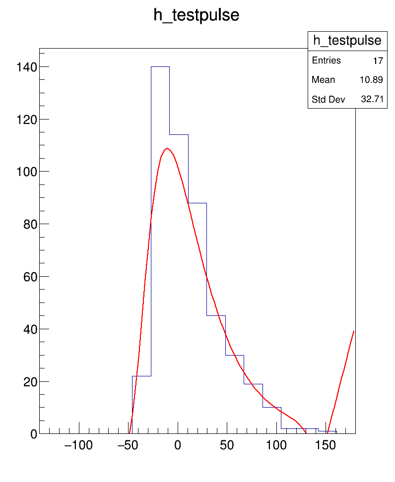
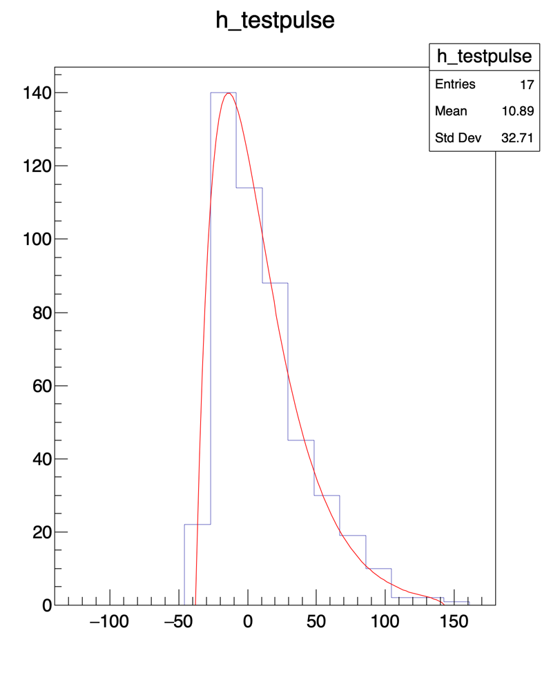
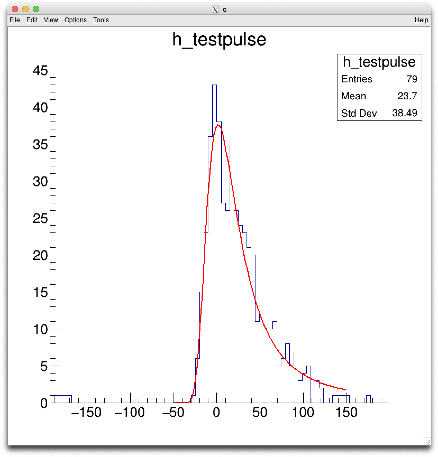
Plot:

[eguiraud]

Hi @eska ,

we need @moneta 's help here, let’s ping him.

Cheers,
Enrico

[moneta]

Hi,
The problem is that you need to fix the amplitude parameter of the Gaussian function or not defining it, otherwise you will have in the fit two multiplicative parameter that will be 100% correlated.
By doing this and setting good initial parameters the fit seems to work. The statistics is very low and you have many parameters, so few degrees of freedom, this also can make the fit not very stable.
You can find a revised version of the macro working for me,

Best regards

Lorenzo

rootForum_52265.C (1.3 KB)

[eska]

Hi Lorenzo,
Thanks a lot for your reply. I see, fixing the amplitude of the Gaussian makes sense.

I tried running your macro, but it seems the fit did not work for me. Was there something I should have modified before? Please find a picture of my output below.

[moneta]

Hi,
Are you sure you are running the code I have attached with those initial parameter values ?
I am getting this result below.
If this is the case can you please post the full output log as well, thank you

Lorenzo

[eska]

I tried again, but I still get the same plot.

Just in case, this is the root I use (currently working on lxplus), maybe that can help finding the cause: /cvmfs/sft.cern.ch/lcg/app/releases/ROOT/6.24.06/x86_64-centos7-gcc48-opt/bin/thisroot.sh

This is my output:

Processing doubleExpWithGauss.C...
Info in <TCanvas::MakeDefCanvas>:  created default TCanvas with name c1
 FCN=199.757 FROM MIGRAD    STATUS=CONVERGED     144 CALLS         145 TOTAL
                     EDM=1.25347e-07    STRATEGY= 1  ERROR MATRIX UNCERTAINTY   0.2 per cent
  EXT PARAMETER                                   STEP         FIRST   
  NO.   NAME      VALUE            ERROR          SIZE      DERIVATIVE 
   1  p0           1.36354e+00   8.04981e-02  -5.92858e-04   7.87144e-02
   2  p1           3.65365e+01   4.39327e-02   2.97623e-04  -5.23939e-03
   3  p2           8.93757e+00   5.56792e-01  -3.71409e-03  -1.19763e-02
   4  p3           9.42013e+05   3.08909e+05  -1.97473e+02   8.92459e-12
   5  p4           1.00000e+00     fixed    
   6  p5           1.64867e+01   9.33302e-02   6.60585e-04  -5.18208e-03

****************************************
Minimizer is Minuit / Migrad
Chi2                      =      199.757
NDf                       =            5
Edm                       =  1.25347e-07
NCalls                    =          145
p0                        =      1.36354   +/-   0.0804981   
p1                        =      36.5365   +/-   0.0439327   
p2                        =      8.93757   +/-   0.556792    
p3                        =       942013   +/-   308909      
p4                        =            1                      	 (fixed)
p5                        =      16.4867   +/-   0.0933302   

Covariance Matrix:

            	          p0          p1          p2          p3          p5
p0          	   0.0064799  -0.0034273    0.044622      2048.6   -0.007453
p1          	  -0.0034273   0.0019301   -0.023775     -1088.1   0.0039626
p2          	    0.044622   -0.023775     0.31002       14116   -0.051544
p3          	      2048.6     -1088.1       14116  9.5425e+10     -2365.5
p5          	   -0.007453   0.0039626   -0.051544     -2365.5   0.0087105

Correlation Matrix:

            	          p0          p1          p2          p3          p5
p0          	           1    -0.96912     0.99557    0.082384    -0.99203
p1          	    -0.96912           1    -0.97192   -0.080176     0.96642
p2          	     0.99557    -0.97192           1    0.082069    -0.99189
p3          	    0.082384   -0.080176    0.082069           1   -0.082047
p5          	    -0.99203     0.96642    -0.99189   -0.082047           1
Info in <TCanvas::Print>: file test.png has been created

[moneta]

Hi,

I can reproduce the problem on lxplus and also another machine. I think there is a fundamental problem in the function definition and how the convolution is performed.
The function to convolute, the double exponential, is not going to zero for large negative x and this makes the convolution integral to diverge.
I think you might need to define the exponential function with something like:

"(x > [4] ) ? [0]*exp(-x/[1])-[2]*exp(-x/[3]) : 0" 

where [4] is an additional fit parameter or you might want to use just zero.
Also your data don’t have the sensitivity for detecting two exponential functions, I would just fit a single one. So using this fitfunction:

   TF1Convolution *f_conv = new TF1Convolution("(x>[2]) ? [0]*exp(-x/[1]) : 0", "[0]*exp(-(x)^2/[1]^2)", \
-50, 150, true);
   f_conv->SetRange(-50., 150.);
   f_conv->SetNofPointsFFT(1000);
   f_conv->SetExtraRange(0.2);

   TF1 *f = new TF1("f", *f_conv, -50., 150., f_conv->GetNpar());

   f->SetParameters(5., 10., 0., 1., 12.8);
   f->FixParameter(3,1);

I don’t know what the data represent, so there could be also a better function to fit them.

Lorenzo

[eska]

Hello,

To provide a bit more context, the aim is to fit the light pulse of a signal coming from scintillating material hitting on a photodetector (the x axis denotes the time of arrival using the moment of interaction of the passing particle with the scintillation material as t_{start}). In fact, the scintillation response is modelled in GEANT4 using a somewhat more constrained version of a double exponential (defined in G4Scintillation.hh):

inline
G4double G4Scintillation::bi_exp(G4double t, G4double tau1, G4double tau2)
{
         return std::exp(-1.0*t/tau2)*(1-std::exp(-1.0*t/tau1))/tau2/tau2*(tau1+tau2);
}

This is how the double exponential comes into play for the convolution (the gaussian is there to account for the fluctuations in time of arrival regardless of the scintillation response). I have tried to use this version of a double exponential as well, but with limited success. It was something that I found strange however, since in principle

e^{-\frac{t}{\tau_2}}\left(1-e^{-\frac{t}{\tau_1}}\right)\frac{\tau_1+\tau_2}{\tau_2^2}

and

A_1e^{-\frac{t}{\tau_1}}+A_2e^{-\frac{t}{\tau_2}}

are the same with the coefficients, if I’m not mistaken, obeying the following equations (although A_i and t_i are not independent):

A_1=-A_2=\frac{\tau_1+\tau_2}{\tau_2^2} and t_1=\tau_2 and t_2=\frac{1}{\tau_1}+\frac{1}{\tau_2}

For the data, I increased the number of bins, but unfortunately the total number of detected events per pulse is very limited (this is stilling missing background noise which would further distort the shape of the distribution) so this is the best one can do as far as I know:

std::vector<double> xvals =    {4437.5, 4442.5, 4447.5, 4452.5, 4457.5, 4462.5, 4467.5, 4472.5, 4477.5, 4482.5, 4487.5, 4492.5, 4497.5, 4502.5, 4507.5, 4512.5, 4517.5, 4522.5, 4527.5, 4532.5, 4537.5, 4542.5, 4547.5, 4552.5, 4557.5, 4562.5, 4567.5, 4572.5, 4577.5, 4582.5, 4587.5, 4592.5, 4597.5, 4602.5, 4607.5, 4612.5, 4617.5, 4622.5, 4627.5, 4632.5, 4637.5, 4642.5, 4647.5, 4652.5, 4657.5, 4662.5, 4667.5, 4672.5, 4677.5, 4682.5, 4687.5, 4692.5, 4697.5, 4702.5, 4707.5, 4712.5, 4717.5, 4722.5, 4727.5, 4732.5, 4737.5, 4742.5, 4747.5, 4752.5, 4757.5, 4762.5, 4767.5, 4772.5, 4777.5, 4782.5, 4787.5, 4792.5, 4797.5, 4802.5, 4807.5, 4812.5, 4817.5, 4822.5, 4827.5};
std::vector<double> yvals =    {     1,      0,    1.0,    1.0,    1.0,    1.0,    0.0,    0.0,    0.0,    0.0,    0.0,    0.0,    0.0,    0.0,    0.0,    0.0,    0.0,    0.0,    0.0,    0.0,    0.0,    0.0,    0.0,    0.0,    0.0,    0.0,    0.0,    0.0,    0.0,    0.0,    0.0,    0.0,    0.0,    0.0,    1.0,    6.0,   15.0,   23.0,   36.0,   43.0,   38.0,   27.0,   26.0,   35.0,   26.0,   24.0,   23.0,   21.0,   20.0,   11.0,   12.0,   12.0,   10.0,   11.0,    5.0,    6.0,    8.0,    5.0,    7.0,    3.0,    4.0,    5.0,    0.0,    3.0,    2.0,    0.0,    0.0,    1.0,    1.0,    1.0,    1.0,    0.0,    0.0,    0.0,    0.0,    1.0,    0.0,    0.0,    0.0};

With noise, the distribution looks like this:

std::vector<double> xvals = {4432.5, 4437.5, 4442.5, 4447.5, 4452.5, 4457.5, 4462.5, 4467.5, 4472.5, 4477.5, 4482.5, 4487.5, 4492.5, 4497.5, 4502.5, 4507.5, 4512.5, 4517.5, 4522.5, 4527.5, 4532.5, 4537.5, 4542.5, 4547.5, 4552.5, 4557.5, 4562.5, 4567.5, 4572.5, 4577.5, 4582.5, 4587.5, 4592.5, 4597.5, 4602.5, 4607.5, 4612.5, 4617.5, 4622.5, 4627.5, 4632.5, 4637.5, 4642.5, 4647.5, 4652.5, 4657.5, 4662.5, 4667.5, 4672.5, 4677.5, 4682.5, 4687.5, 4692.5, 4697.5, 4702.5, 4707.5, 4712.5, 4717.5, 4722.5, 4727.5, 4732.5, 4737.5, 4742.5, 4747.5, 4752.5, 4757.5, 4762.5, 4767.5, 4772.5, 4777.5, 4782.5, 4787.5, 4792.5, 4797.5, 4802.5, 4807.5, 4812.5, 4817.5, 4822.5, 4827.5};
std::vector<double> yvals = {32.0, 58.0, 40.0, 43.0, 45.0, 44.0, 43.0, 51.0, 38.0, 42.0, 46.0, 33.0, 35.0, 46.0, 34.0, 40.0, 40.0, 39.0, 41.0, 40.0, 40.0, 54.0, 34.0, 52.0, 51.0, 46.0, 40.0, 36.0, 49.0, 38.0, 33.0, 42.0, 35.0, 35.0, 41.0, 30.0, 56.0, 52.0, 66.0, 86.0, 82.0, 79.0, 68.0, 63.0, 76.0, 70.0, 77.0, 63.0, 58.0, 62.0, 57.0, 43.0, 53.0, 51.0, 62.0, 64.0, 60.0, 55.0, 52.0, 46.0, 48.0, 52.0, 35.0, 43.0, 44.0, 36.0, 41.0, 50.0, 55.0, 41.0, 51.0, 32.0, 55.0, 44.0, 41.0, 41.0, 35.0, 49.0, 36.0, 38.0};

Edit: Like before, the time array values are shifted by 4630 to simplify the fit as that removes the necessity to account for the peak position along the time axis.

[moneta]

Hi,

I understand it better now. It is clear then that you have to define your exponential function to be equal to zero for t < t_start , the time of arrival of the particle with the detector. You might fit this value in the data as I have shown in the previous post.

Lorenzo

[eska]

Hi Lorenzo,

Sorry for the delayed reply. I tried doing this, but unfortunately, without success. I tried with these definitions of the convolution:

TF1Convolution *f_conv = new TF1Convolution("(x > 0) ? exp(-x/[0])/([0]) : 0", "(x>0) ? [0]*exp(-(x-[1])^2/[2]^2) : 0", -50, 150, true);

TF1Convolution *f_conv = new TF1Convolution("(x > 0) ? expo : 0", "(x>0) ? gaus : 0", -50, 150, true);

TF1Convolution *f_conv = new TF1Convolution("expo", "gaus", -50, 150, true);

Followed by these parameter constraints

f_conv->SetRange(-50., 150.);
f_conv->SetNofPointsFFT(1000);
f_conv->SetExtraRange(0.2);
   
TF1 *f = new TF1("f", *f_conv, -50., 150., f_conv->GetNpar());
   
f->SetParLimits(0, 1., 30);
f->SetParLimits(1, 10, 10000000);
f->SetParLimits(2, -20,20);
f->SetParLimits(3, 0.5, 20);
	
f->SetParameters(16., 1000, 0., 1.);

I added parameter limits as well, but it did not help.

As I have begun doubting the suitability of the chosen functions as you also initially suggested, I have tried to fit a Landau, since it just “looked” quite like a Landau distribution, and indeed the result is basically perfect:

What concerns me is that based on my previous argumentation, physically, the distrubtion should follow a convolution of a (bi-) exponential with another function, presumably Gaussian. I have no physical explanation as to why this distribution should follow a Landau. I was also able to somewhat fit a convolution using Python’s curve_fit module, and adding to that the quite good result you shared at the beginning of this post, I took this as evidence that the convolution should work and only needed some tweaking. But I may have been mistaken about that.

In any case, I appreciate your help, since it gave me more insight into fitting with ROOT. Thanks a lot and sorry for the inconvenience.