Bugs in ROOT using Jupyter Notebooks?

Hi there, I am a very new ROOT user (working as a summer student) and someone I am working with who is very versed in ROOT and Python thinks there is a bug in the version of ROOT that runs through Jupyter notebooks.

The two issues we have run into are:
[ul]1. While having three 2D histograms overlaid onto one plot using TGraph and TMultiGraph, the legend will not appear.[/ul]
[ul]2. While having three 1D histograms overlaid, it is not possible to show more than one Gaussian fit.[/ul]

Samples of the code (a bit simplified) are found below:

1. Missing Legend

plot1 = ROOT.TGraph(n,Time1,Amp1) mg = ROOT.TMultiGraph() mg.Add(plot1) leg = ROOT.TLegend(0.5,0.5,0.5,0.5) leg.SetHeader("Legend") leg.AddEntry(plot1,path1,"2") leg.Draw() c1.Draw()

This code was adjusted to accommodate three 2D histograms in total. The legend for this graph will not appear.

2. Missing Gaussian Fits

h1 = ROOT.TH1F("h1","Normalized Amplitude Histogram",1000,0,3000) tree.Draw("fPulseData[0].GetParameter(0)>>h1") gfit1 = ROOT.TF1("gfit1","gaus(0)",1000,1800) gfit1.SetParameters(100,150,1000,0,0) h1.Scale(1./h1.Integral()) h1.Fit(gfit1,"rme") h1.Draw() gfit1.Draw("same") c1.Draw()

This code was adjusted to accommodate three histograms and three Gaussian fits in total.The problem is that it only plots the last-called Gaussian fit (in black)- the other two do not show up on the graph even though their statistics have been calculated.

Does anyone else experience this issue in Jupyter Notebooks? I understand that it is fairly new so there are bound to be some bugs. On the other hand, if I am doing something wrong, please let me know.

Thanks very much!

Hi,

welcome to the ROOT forum!
I simplified your two examples and made them standalone for future reference.

  1. Legend:
    Here the problem is that you created a “pointlike” legend. You set the lower right and upper left corners’ coordinates to (0.5,0.5). Here you can find a solution to your issue (also incorporating the header in the legend constructor)
import ROOT
import array

Time1=array.array('d',[x for x in xrange(10)])
Amp1=array.array('d',[x*x for x in xrange(10)])
n=len(Amp1)
plot1 = ROOT.TGraph(n,Time1,Amp1)
plot1.SetMarkerStyle(22)

mg = ROOT.TMultiGraph()
mg.Add(plot1)

# Important line
leg = ROOT.TLegend(.8,.8,1,1,"Legend")
path1="lala"
leg.AddEntry(plot1,path1)

c1=ROOT.TCanvas()
plot1.Draw("AP")
leg.Draw("Same")
c1.Draw()
  1. Fit functions not displayed
    I suspect you are fitting with the same function object the histograms. While mathematically this is perfectly sane, as you say the parameters are printed, in the program the function, and therefore the line on the canvas, is only one. Here you can find a proposal which uses 3 gaussians.
import ROOT

h1=ROOT.TH1F("h1","h1",64,-4,4)
h2=ROOT.TH1F("h2","h2",64,-4,4)
h3=ROOT.TH1F("h3","h3",64,-4,4)

# make them different
for h,s in zip([h1,h2,h3],[1,1.5,2]):
    h.FillRandom("gaus")
    h.Scale(s)

gfit1 = ROOT.TF1("gfit1","gaus(0)",-4,4)
gfit2 = ROOT.TF1("gfit2","gaus(0)",-4,4)
gfit3 = ROOT.TF1("gfit3","gaus(0)",-4,4)

h1.Fit(gfit1,"rme")
h2.Fit(gfit2,"rme")
h3.Fit(gfit3,"rme")


c=ROOT.TCanvas()
h3.Draw()
h2.Draw("Same")
h1.Draw("Same")
c.Draw()

Good luck with your internship :slight_smile:

Cheers,
D

[quote=“dpiparo”]
2. Fit functions not displayed
I suspect you are fitting with the same function object the histograms. While mathematically this is perfectly sane, as you say the parameters are printed, in the program the function, and therefore the line on the canvas, is only one. Here you can find a proposal which uses 3 gaussians.

import ROOT

h1=ROOT.TH1F("h1","h1",64,-4,4)
h2=ROOT.TH1F("h2","h2",64,-4,4)
h3=ROOT.TH1F("h3","h3",64,-4,4)

# make them different
for h,s in zip([h1,h2,h3],[1,1.5,2]):
    h.FillRandom("gaus")
    h.Scale(s)

gfit1 = ROOT.TF1("gfit1","gaus(0)",-4,4)
gfit2 = ROOT.TF1("gfit2","gaus(0)",-4,4)
gfit3 = ROOT.TF1("gfit3","gaus(0)",-4,4)

h1.Fit(gfit1,"rme")
h2.Fit(gfit2,"rme")
h3.Fit(gfit3,"rme")


c=ROOT.TCanvas()
h3.Draw()
h2.Draw("Same")
h1.Draw("Same")
c.Draw()

Good luck with your internship :slight_smile:

Cheers,
D[/quote]

Hi there, thanks for your quick response. I have tried your suggestions and here are my results:

[ul]1. Your legend solution worked mostly - thanks! The only issue is that the colours of the plots do not show up on the legend. I have tried fixing this with no results.[/ul]

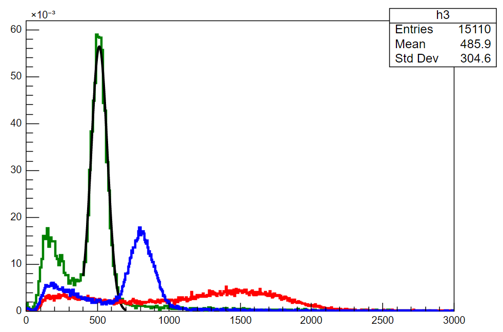
[ul]2. Your Gaussian solution seems to not have worked. I have provided a full copy of the code written by my colleague that gives the plot provided in my first post - as far as I can see, it is identical to the solution you provided sans the for-loop. I ran the code you provided, and like ours, it only plots the last-called Gaussian, gfit3. Could you elaborate on what exactly the for-loop is intending to do? It seems to arbitrarily scale them based on the tuple you make using zip(), which removes valuable information to us about the data. In our code below you can see that we have normalized our histograms so that we can compare them. [/ul]

[code]import ROOT
import pylab as pl
import numpy as np
ROOT.enableJSVis()
c1 = ROOT.TCanvas()
%matplotlib inline

Load our custom filters

ROOT.gSystem.Load("/usr/local/software/quadis/latest/quadis/build/lib/libquadis.so")

These are the names of our data files:

path1='qe12f000’
path2='qe12f001’
path3=‘qe12f002’

These are the locations of our data files to import and set pointers:

infile = ROOT.TFile("/data/news/queens/T1/"+path1+".root")
infile2 = ROOT.TFile("/data/news/queens/T1/"+path2+".root")
infile3 = ROOT.TFile("/data/news/queens/T1/"+path3+".root")
tree = infile.Get(“T1”)
tree2 = infile2.Get(“T1”)
tree3 = infile3.Get(“T1”)
tree.GetEntry()
tree2.GetEntry()
tree3.GetEntry()
nevent = ROOT.NEvent()
nevent2 = ROOT.NEvent()
nevent3 = ROOT.NEvent()
tree.SetBranchAddress(“NEvent”,nevent)
tree2.SetBranchAddress(“NEvent”,nevent2)
tree3.SetBranchAddress(“NEvent”,nevent3)

h1 = ROOT.TH1F(“h1”,“Normalized Amplitude Histogram”,1000,0,3000) #set range of h1
h2 = ROOT.TH1F(“h2”,“Normalized Amplitude Histogram”,1000,0,3000) #set range of h2
h3 = ROOT.TH1F(“h3”,“Normalized Amplitude Histogram”,1000,0,3000) #set range of h3

tree.Draw(“fPulseData[0].GetParameter(0)>>h1”)
tree2.Draw(“fPulseData[0].GetParameter(0)>>h2”)
tree3.Draw(“fPulseData[0].GetParameter(0)>>h3”)

gfit1 = ROOT.TF1(“gfit1”,“gaus(0)”,1000,1800)
gfit1.SetParameters(100,1500,1000,0,0)

gfit2 = ROOT.TF1(“gfit2”,“gaus(0)”,650,1000)
gfit2.SetParameters(100,750,500)

gfit3 = ROOT.TF1(“gfit3”,“gaus(0)”,400,700)
gfit3.SetParameters(100,500,500)

gfit1.SetLineColor(1)
gfit2.SetLineColor(1)
gfit3.SetLineColor(1)

Normalize all histograms

h1.Scale(1./h1.Integral())
h2.Scale(1./h2.Integral())
h3.Scale(1./h3.Integral())

h1.SetLineColor(2)
h2.SetLineColor(4)
h3.SetLineColor(3)

h1.Fit(gfit1,“rme”)
h2.Fit(gfit2,“rme”)
h3.Fit(gfit3,“rme”)

h3.Draw()
h1.Draw(“same”)
h2.Draw(“same”)

gfit1.Draw(“same”)
gfit2.Draw(“same”)
gfit3.Draw(“same”)
c1.Draw()
[/code]

Thanks again!

Hi,

About the legend, I cannot reproduce the issue: if I take this code and run it in a cell, I get the correct marker and line colours in the legend:

import ROOT
import array
%jsroot on
Time1=array.array('d',[x for x in xrange(10)])
Amp1=array.array('d',[x*x for x in xrange(10)])
n=len(Amp1)
plot1 = ROOT.TGraph(n,Time1,Amp1)
plot1.SetMarkerStyle(22)
plot1.SetMarkerSize(2)
plot1.SetFillColor(ROOT.kWhite)
plot1.SetLineColor(ROOT.kRed)

mg = ROOT.TMultiGraph()
mg.Add(plot1)

# Important line
leg = ROOT.TLegend(.8,.8,1,1,"Legend")
path1="lala"
leg.AddEntry(plot1,path1)

c1=ROOT.TCanvas()
mg.Draw("APL")
leg.Draw("Same")
c1.Draw()

This was a simple artifact to create histograms randomly filled: I would not be distracted by it. Below I made the example you shared standalone (I cannot access your library and trees).
The missing lines are due to an hiccup in the javascript based visualisation. The expert is informed. Waiting for a fix, I can suggest a workaround, i.e. to switch to regular visualisation for this particular plot.

import ROOT
#ROOT.enableJSVis()
c1 = ROOT.TCanvas()

h1 = ROOT.TH1F("h1","Normalized Amplitude Histogram",100,0,3) #set range of h1
h2 = ROOT.TH1F("h2","Normalized Amplitude Histogram",100,0,3) #set range of h2
h3 = ROOT.TH1F("h3","Normalized Amplitude Histogram",100,0,3) #set range of h3

h1.FillRandom("gaus")
h2.FillRandom("gaus")
h3.FillRandom("gaus")

gfit1 = ROOT.TF1("gfit1","gaus(0)",0,3)
gfit2 = ROOT.TF1("gfit2","gaus(0)",0,3)
gfit3 = ROOT.TF1("gfit3","gaus(0)",0,3)

gfit1.SetLineColor(1)
gfit2.SetLineColor(1)
gfit3.SetLineColor(1)

# Normalize all histograms
h1.Scale(1./h1.Integral())
h2.Scale(1./h2.Integral())
h3.Scale(1./h3.Integral())

h1.SetLineColor(2)
h2.SetLineColor(4)
h3.SetLineColor(3)

h1.Fit(gfit1,"rme")
h2.Fit(gfit2,"rme")
h3.Fit(gfit3,"rme")

h3.Draw()
h1.Draw("same")
h2.Draw("same")

gfit1.Draw("same")
gfit2.Draw("same")
gfit3.Draw("same")
c1.Draw()

Cheers,
Danilo